 Open Journal of Statistics, 2012, 2, 153-162 http://dx.doi.org/10.4236/ojs.2012.22017 Published Online April 2012 (http://www.SciRP.org/journal/ojs) 153 A Universal Selection Method in Linear Regression Models Eckhard Liebscher Department of Computer Science and Communication Systems, Merseburg University of Applied Sciences, Merseburg, Germany Email: eckhard.liebscher@hs-merseburg.de Received January 27, 2012; revised February 29, 2012; accepted March 9, 2012 ABSTRACT In this paper we consider a linear regression model with fixed design. A new rule for the selection of a relevant sub- model is introduced on the basis of parameter tests. One particular feature of the rule is that subjective grading of the model complexity can be incorporated. We provide bounds for the mis-selection error. Simulations show that by using the proposed selection rule, the mis-selection error can be controlled uniformly. Keywords: Linear Regression; Model Selection; Multiple Tests 1. Introduction In this paper we consider a linear regression model with fixed design and deal with the problem of how to select a model from a family of models which fits the data well. The restriction to linear models is done for the sake of transparency. In applications the analyst is very often interested in simple models because these can be inter- preted more easily. Thus a more precise formulation of our goal is to find the simplest model which fits the data reasonably well. We establish a principle for selecting this “best” model. Over time the problem of model selection has been studied by a large number of authors. The papers [1,2] by Akaike and Mallows inspired statisticians to think about the comparisons of fitted models to a given dataset. Akaike, Mallows and later Schwarz (in [3]) developed information criteria which may be used for comparisons and in particular, may be applied to non-nested sets of models. The basic idea is the assessment of the trade-off between the improved fit of a larger model and the in- creased number of parameters. Akaike’s approach is to penalise the maximised log-likelihood by twice the num- ber of parameters in the model. The resulted quantity, the so called AIC, is maximised with respect to the parame- ters and the models. The disadvantage of this procedure is that it is not consistent; more precisely, the probability of overfitting the model tends to a positive value. Subse- quently, a lot of other criteria have been developed. In a series of papers the consistency of procedures based on several information criteria (BIC, GIC, MDL, for exam- ple) are shown. The MDL-method was introduced by Rissanen in [4]. In the nineties of the last century a new class of model selection methods came into focus. The FDR procedure of Benjamini and Hochberg (see [5]) uses ideas from multiple testing and attempts to control the false discovery rate, which we will call the mis-se- lection rate in this paper. More recent papers of this di- rection are published by Bunea et al. [6], and by Benja- mini and Gavrilov [7]. Surveys of the theory and existing results may be found in [8-11]. In a large number of pa- pers the consistency and loss efficiency of the selection procedure is shown and the signal to noise ratio is calcu- lated for the criterion under consideration. Among these papers we refer to [12-16], where consistency is proved in a rather general framework. A method for the sub- model selection using graphs is studied in [17]. Leeb and Pötscher examine several aspects of the post-model-se- lection inference in [9,18,19]. The authors point out and illustrate the important distinction between asymptotic results and the small sample performance. Shao intro- duced in [20] a generalised information criterion, which includes many popular criteria or which is asymptotically equivalent to them. In this paper Shao proved conver- gence rates for the probability of mis-selection. In [21] a rather general approach using a penalised maximum like- lihood criterion was considered for nested models. Edwards and Havránek proposed in [22] a selection procedure aimed at finding sets of simplest models that are accepted by a test like a goodness-of-fit test. Unfor- tunately, it is not possible to use the typical statistical tests of linear models in Edwards and Havránek’s proce- dure since the assumption (b) in the Section 2 of their paper is not fulfilled (cf. Section 4 of their paper). In this paper we develop a new universal method for selecting a significant submodel from a linear regression model with fixed design, where the selection is done C opyright © 2012 SciRes. OJS  E. LIEBSCHER 154 from the whole set of all submodels. We point out the several new features of our approach: 1) A new selection procedure based on parameter tests is introduced. The procedure is not comparable with methods based on information criteria and it is different from Efroymson’s algorithm of stepwise variable selec- tion in [23]. 2) We derive convergence rates for the probability of mis-selection which are better than those proved in pa- pers about information criteria e.g. in [20]. 3) Subjective grading of the model complexity can be incorporated. Concerning 1) we consider tests on a set of parameters in contrast to FDR-methods, where several tests on only one parameter are applied. Moreover w.r.t. 2), many au- thors do not analyse the behaviour of mis-selection pro- babilities. The results on bounds or convergence rates of these probabilities are more informative than the consis- tency. The aspect 3) is of special interest from the point of view of model building. Typically model builder have some preference rules in mind when selecting the model. They prefer simple models with linear functions to mod- els with more complex functions (exponential or loga- rithmic, for example). The crucial idea is to assign to each submodel a specific complexity number. We do not assume that the errors are normally distrib- uted. This ensures a wide-ranging applicability of the approach, but only asymptotic distributions of test statis- tics are available. From examples in Section 2, it can be seen that applications are possible in several directions, for instance to the one-factor-ANOVA model. The simu- lations show an advantage of the proposed method in that it controls the frequency of mis-selection uniformly. For models with a large number of regressors, the problem of establishing an effective selection algorithm is not dis- cussed in this paper; we refer to the paper [24]. The paper is organised as follows: In Section 2 we in- troduce the regression model and several versions of submodels. The asymptotic behaviour of the basic statis- tic is also studied there. Section 3 is devoted to the model selection method. We provide convergence rates for the probability that the procedure selects the wrong model (mis-selection). We see that the behaviour is similar to that in the case of hypothesis testing. The results of simu- lations are discussed in Section 4. The reader finds the proofs in Section 5. 2. Models Let us introduce the master model 1 k i j iijj Yx 1, ,in 1,, nk jk 1,, Tk ,, n for , where is the design matrix, k is the parameter vector, and 1 1,, , ij in Xx 0 i are independent random variables. Assume that , p i 2p for some , and 2 Var i . 1n denote the values of the re- sponse variable. In short we can write ,,YY YX ,, T YY Y 1,, T n , (1) where 1n, . The least square estimator for is given by 1 ˆTT XXY . This leads to the residual sum of squares 21 ˆTTT n RYX YIXXXXY , where is the Euclidean vector norm. . The aim is to select model (1) or an appropriate sub- model which fits the data well. Moreover, we search for a reasonably simple model. In the following we define the submodels of (1). The submodel with index 1, , ,,, Tl l :ll has the parameter vector 12 , , where the vector is related to by D with an appropriate ma- trix kl D lk having maximum rank . In a large number of applications, the γi’s coincide with different components of . The submodel indices 1 and correspond to the model function equal to zero (no pa- rameters) and to the full model, respectively. Thus we can write the model equation for the submodel as YX , (2) XD . The parameter space of submodel where in (1) is given by :l D . Next we give several versions for the definition of submodels in dif- ferent situations. Example 1. We consider all submodels, where com- ponents of are zero. More precisely, index is assigned to a submodel if 1 1,, l ili 12 l i 0 j are the parameters of the submodel (ii), for 1 :,, l jJi i 1 1 12 j li j 0,,0,1,0,Tk ii e and . Let be the i-th unit vector. Then 12 ,,, l kl ii i Dee e , and :0 for all jjJ 5k . For example, for , the submodel with index 14 has the parameters 11 , 23 , 34 and 25 0 100 000 010 001 000 D 5 25 :0 holds. Moreover, we have , Copyright © 2012 SciRes. OJS  E. LIEBSCHER 155 in this case. Here the digits “1” in the binary representa- tion of 1 give the indices of the parameters available in the submodel . in (2) consists of the columns 1l of the design matrix ,i,i correspond- ing to the present parameters in submodel . □ Example 2. Let . submodel 1: 3k10 T , 23. Submodel 2: , 11 , . Sub- model 3: identity (1). □ 23 ,T ij Y Example 3. We consider the one-factor ANOVA model i ij for , 1, ,ig1, , jn ,g Tn ngn Y ,, k , where , 11 12121 1 ,,, ,,YYYYY gT 1i nn ,, i, 1g is the parameter vector. 11 n are independent random variables. The submodels are characterised by the fact that several μi’s are equal. Let be the k-th Bell number. A Sub- model with index 1, , is determined by a par- tition 1, ,, l JJ of 1, , for some ii in the following way: , jk jk J : i f . The submodel with index has l parameters. Furthermore, 1,, , ij ik Dd 1 where 0 o 1,,holds jl for , therwise. , ij d iJ □ Example 3 shows that the model selection problem occurs also in the context of ANOVA. In submodel (2) with index , the least square estimator ˆ and the residual sum of squares S are given by 1. T X XY : n 1 2 ˆ, ˆ TT TT XX XY SYX YIXX (3) What is an appropriate statistic for model selection? Let n SR . Here we consider a quantity n M , which is similar to F-statistics known from hy- pothesis testing in linear regression models with normal errors: 1 ˆ 1 for , 0. n n TT n M M S nl DX nl M ˆˆ ˆ XD S (4) The main difference to classical F-statistics is that the estimator 1S nl of the model variance in submodel appears in the denominator. The quantity 1S nl is the proper estimator under the hypothesis of submodel . Classical F-statistics are used in Efroymson’s algo- rithm of stepwise variable selection (see [23]). In the remainder of this section we study the asymp- totic behaviour of the statistic M when 0n is the true parameter of the model (1). For this reason, we first introduce some assumptions. Assumption . Let 1T n GXX n . Assume that Rank n Gk , lim n nG , regular. Moreover, 2 1, ,1 :max. npp np ij jk i Bxon ij □ In a wide range of applications, the entries of the design matrix are uniformly bounded such that 2p np BOnon 2p :ll T DD since . The Assumption may be weakened in some ways, but we use this as- sumption to reduce the technical effort. We introduce and 1 00 :TT KIDD . Proposition 2.1 clarifies the asymptotic behaviour of the statistic Mn. Proposition 2.1. Assume that Assumption is sat- isfied. 0 1) Assume that lk and . Then we have 2 nkl M . 2) Suppose that 0 k and l. Let 12 n Gon be satisfied n. Then we have 1 2 nn KKnnWon , 2 0, nW W where 2 22 2 4 W , K . Depending on whether the true parameter 0 belongs to submodel or not, the statistic Mn has a dif- ferent asymptotic behaviour. In the first case, it has an asymptotic χ2-distribution. In the second case it tends to infinity in probability with rate n. Therefore, the sta- tistic Mn is suitable for model selection. In the next section a selection procedure is introduced based on n M serving as fundamental statistic. 3. The New Selection Rule In this section we propose a selection rule which is based Copyright © 2012 SciRes. OJS  E. LIEBSCHER yright © 2012 Sc OJS 156 d dd are: on the statistic (4). We introduce a measure d 1) is the degree of the polynomial plus 1, of the complexity for submodel with max . With this quantity dl dd d02) is the number of parameters avail- able in the submodel, the other parameters it is possible to incorporate a subjective grading of the model com- plexity. The restriction to integers is made for simpler handling in the selection algorithm. The following exam- ples should illustrate the applicability of the complexity measure. are zero, CopiRes. Example 4. We consider the polynomial k. The regressor is observed at the measurement points 1 12 px 1k x x ,, n x. Hence 1 ij i x k or , . Possible choices for f1, ,in1, ,j 3) 1 2 kk dl l, where is the number of parameters available in the submodel. This choice has the advantage that a polynom of higher degree al- ways gets a higher complexity number. □ Example 5. For a quasilinear model with regression function 12 3 ln xxx d, we can define as follows: 12 3 12 132 3 1 for submodel functions ,, 2 for submodel function ln odel function bmodel functions ln,ln 5 for the full model fxfxx fx x dfx x3 for 4 fo subm r su xxfxxx :, \i iii d This choice takes into account that the logarithm is a more complex function in comparison to constants or linear functions. □ Next we need restricted parameter sets defined by d . It is assumed that for . 1, , dl Example 1: If then :0 for all ,0 for all jj jJ jJ l . □ d Example 3: If then : for all ,,, if , for some jki Ijki jJkJiIjkJ i . □ Given values max 0, ,0, nn d , 1 , we introduce special χ2-quantiles: 2 ,1 nkln dl d 0, ,1lk ,1 ndk ,dl for , . Here n is just the quantile of order 1d n of the asymptotic distribution of Mn unter the null hypothesis 0 d , cf. part 1) of Proposition 2.1. The quantity n will play the role of an asymptotic type-1 error probability later. A submodel is referred to as admissible if ,Mdl nn is satisfied, which in turn corresponds to the nonrejection of the hy- pothesis that the parameter belongs to the space of the submodel. The generalised information criterion in- troduced by Shao (see [20]) is given by nn GIC Sl Rn k. We next show that there is a relationship between the both approaches. A sub- model is admissible if GIC GIC , where nn n . More- over, note that our selection procedure is completely dif- ferent from Shao’s one. Whereas n nk klnk in information criteria is typically free of choice, the quantity n is well-defined and motivated. Let l be the distribution function of the -distribution. We introduce the fol- lowing rule for the selection: Select a model ν* such that 2 l *min :1,, nn dd Mdl and * * * min:1 ,. n kl n kl FM FMd d The central idea is to prefer any admissible model with lower complexity. If there is more than one admissible model with the same minimum complexity, then we take the model with maximum p-value of M. n The next step is to analyse the asymptotic behaviour of the probability that the wrong model is selected; i.e. the probability of mis-selection (PMS). Let 0 , dd , ll . The following cases of mis-selec- tion can occur: (m1) , nn dl , (m2) , nn dl , nn kli kl FMiFM for some :idi d, nn Mj M for all :jdjd, (m3) , nn , nn dl , jdjlj 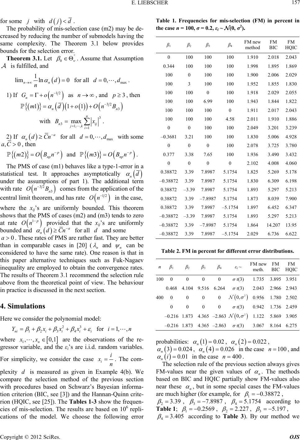 E. LIEBSCHER 157 for some with jdj d 0 . The probability of mis-selection case (m2) may be de- creased by reducing the number of submodels having the same complexity. The Theorem 3.1 below provides bounds for the selection error. Theorem 3.1. Let . Assume that Assumption is fulfilled, and 0 n d 1 lim ln n n max 0, , for all dd. 1) If 12 3p n Gon as , and , then n 32 3 111 nn mdoOnB with 3 1, ,1 max n nij jk i Bx 3. 2) If a n for all d with some dCn max 0,, d ,aC0, then 2 np Bn 3mO and np mOBn . The PMS of case (m1) behaves like a type-1-error in a statistical test. It approaches asymptotically d n under the assumptions of part 1). The additional term with rate 32 n On B 3 comes from the application of the central limit theorem, and has rate 12 On 1 in the case, where the xij’s are uniformly bounded. This theorem shows that the PMS of cases (m2) and (m3) tends to zero at rate On provided that the xij’s are uniformly bounded and a dCn d n for all and some . These rates of PMS are rather fast. They are better than in comparable cases in [20] (n 0a and n can be considered to have the same rate). One reason is that in this paper alternative techniques such as Fuk-Nagaev inequality are employed to obtain the convergence rates. The results of Theorem 3.1 recommend the selection rule above from the theoretical point of view. The behaviour in practice is discussed in the next section. 4. Simulations Here we consider the polynomial model: 23 4i i xx 12ni i Yx 3i for 1, ,in where 1n are the observations of the re- gressor variable, and the εi’s are i.i.d. random variables. ,, 0,1xx For simplicity, we consider the case i i xn d . The com- plexity is measured as given in Example 4(b). We compare the selection method of the previous section with procedures based on Schwarz’s Bayesian informa- tion criterion (BIC, see [3]) and the Hannan-Quinn crite- rion (HQIC, see [25]). The Tables 1-3 show the frequen- cies of mis-selection. The results are based on 106 repli- cations of the model. We choose the following error Table 1. Frequencies for mis-selection (FM) in percent in the case n = 100, σ = 0.2, εi ~ (0, σ2). β1 β2 β3 β4 FM new method FM BIC FM HQIC 0 100100 100 1.910 2.0182.043 0.344 100 100 100 1.998 1.8951.869 100 0 100 100 1.900 2.0062.029 100 3 100 100 1.952 1.8551.830 100 1000 100 1.918 2.0292.055 100 1006.99 100 1.943 1.8441.822 100 100100 0 1.911 2.0172.043 100 100100 4.58 2.011 1.9101.886 0 0 100 100 2.049 3.2013.239 –0.36813.21100 100 1.830 5.0064.928 0 0 0 100 2.078 3.7253.780 0.377 3.387.65 100 1.936 3.4903.432 0 0 0 0 2.102 4.0084.060 0.388723.397.89875.1754 1.825 5.2695.178 –0.388723.397.89875.1754 1.830 6.3096.198 0.38872–3.397.89875.1754 1.893 5.2975.213 0.388723.39–7.89875.1754 1.873 8.0397.900 0.388723.397.8987–5.1754 1.897 6.4526.347 –0.38872–3.397.89875.1754 1.893 5.2975.213 –0.388723.39–7.89875.1754 1.864 14.20713.95 –0.38872 3.397.8987–5.1754 2.029 6.7366.622 Table 2. FM in percent for different error distributions. nβ1 β2 β3 β4 εi ~ FM new meth. FM BIC FM HQIC 1000 0 0 0 σ·t(3) 1.735 3.8953.951 0.4684.104 9.516 6.264σ·t(3) 2.043 2.9662.943 4000 0 0 0 2 0, 0 0 0 0 σ·) 0.942 1.7362.459 –0.2161.8734.365–2.863 0.956 1.7802.502 t(3 2 0, σ·t3) 1.122 5.8693.905 –0.216 1.8734.365–2.863 (3.067 8.1646.275 robpabilities: 10.02, n n, 2 0.022 30.024 n 4 0 n in the case 100.026 n , , and 0.01i 0. Thule of the prevous section alwas FM nin the case 40n e selection riys give -values near the given values of n . The methods based on BIC and HQIC partially show FM-values also near these n , but in some special cases the FM-values are much higher (for example, for 10.38872 , 23.39 , 37.8987 , 45.1754 according to Table 1; 10.2569 , 22.227 5.197, 3 , 5 43.40 according Taur method we to ble 3). By o Copyright © 2012 SciRes. OJS 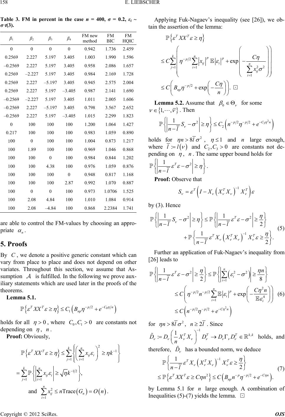 E. LIEBSCHER 158 Table 3. Fin =, εi ~ M in percent the case n 400, σ = 0.2 σ·t(3). 234 method BIC HQIC β1 β β β FM new FM FM 0 0 0 0 0.942 1.7362.459 0.2569 2.227 5.197 3.405 –0.2569 2.227 5.197 3. 1 1 1 1 2 – 1.003 1.9901.596 405 0.958 2.0861.657 0.2569 –2.227 5.197 3.405 0.984 2.1691.728 0.2569 2.227 –5.197 3.405 0.945 2.5752.004 0.2569 2.227 5.197 –3.4050.987 2.1411.690 –0.2569 –2.227 5.197 3.405 1.011 2.0051.606 –0.2569 2.227 –5.197 3.405 0.798 3.5672.652 –0.2569 2.227 5.197 –3.4051.015 2.2991.823 0 100 100 100 1.200 1.0641.427 0.217 100 100 100 0.983 1.0590.890 00 0 100 100 1.004 0.8731.217 100 1.89 100 100 0.969 1.0460.868 100 000 100 0.984 0.8441.202 100 100 4.38 100 0.976 1.0590.876 100 100 000 0.948 0.8171.168 100 100 100 2.87 0.992 1.0700.887 100 0 0 000.973 1.07061.525 100 2.08 4.84 100 1.010 1.0840.914 100 .084.84100 0.868 2.23841.741 are toolMes o - riate able contr the F-valuby chosing an appro pn . of enote a positive generic constant which can ace to place and does not depend on other ate 5. Pros By C, we d vary from pl varis. Throughout this section, we assume that As- sumption is fulfilled. In the following we prove aux- iliary statements which are used later in the proofs of the theorems. Lemma 5.1. 0 2Cn pe or all 1 TT np C B XX holds f0 , wher e 01 ,0CC are constants not ng ondependi , n. Proof: Obvy, iousl 2 1 , kn ij i ji kn ij i ji 11 12 11 TT X xk xk n and 2 1 Trace n ij i nGOn. Applyingaev’s inequality (see [2ob- tain the ass of the lemma: Fuk-Nag6]), we ertion 2 22 11 1 2 exp exp. kn pp p ij in ji ij i p np C Cx x C CB n Lemma 5.2. Assume that 0 TT XX for some 1, , . Then 2 n p n nl holds for 2 3 222 1C p SCe 2 8nl , 1 and n large enough, where :ll and 23 ,0CC are constants note- d pending on , n. The same upper bound holds for 2 1 nl T . Proof: Observe that 1 TTT SIXXXX by (3). Hence 22 1 11 2 1 . 2 T TT T nl XXX X nl S nl (5) Further an application of Fuk-Nagaev’s inequality fro [26] leads to m 2 1 2 22 4 1 22 28 exp i np pp i ii pp Cn Cn Cn Cn e 222 1n T i n nl (6) for 2 8nl , 2nl. Since 1 , 1 :TT Tkk DD XX DDD n holds, and therefore, D has a bounded norm, we deduce 1 22 1 . TT T TTpp Cn np XXX X l XXCnC B ne (7) by Lemma 5.1 for n large enough. A combination of Inequalities (5)-(7) yields the lemma. 2 n Copyright © 2012 SciRes. OJS  E. LIEBSCHER Copyright © 2012 SOJS 159 Note that 00 XX ciRes. 1 2, TTT SXIXXX SSS 12 3 (8) 1 TT XXX where 1 T SIX , 1TTT nn DGDX 20 SIG , 0nn SnGG 1 0 TT n n DGDG 3 , 1 :T n GXX n . 0 Lemma 5.3. Suppose that for some 1, , 2 02K . Let , ll . Then 1) 3 SnKon and 2) 2 2 2 25 40 1pCn p SCn e nl 0 for n 45 ,0CCn and large enough with constants not depending on , . Proof: Part 1) is a consequence of n G and . 2) Using Lemmas 5.1 and 5.2, we deduce n G 13 23 12 12 2 11 11 22 22 11 11 222 2 2 1 2 TT T SSS SS nl nlnl KnCKnCCX l nl nl 0 1 n 22 00 22 0 22 2 2 0 00 1 2 TT pp Cn Cn Tp p np XX Cn CBne Cne nl for 2nl large enouplies assertion 2) of the lemma. An application of thmit theorem and the Cramér-Wold device leads to the following lemma: gh. This im e central li Lemma 5.4. Let 12 :T nnX . i denotes the i-th column of T . Then 2 1 10, n nii i x n . In the second part of this section we provide the proofs of Proposition 2.1 and Theorem 3.1. Proof of Propositio n 2.1. 1) Let 0 . hen D l T00 holds with an appropriate vector 0 . We have 11 1 11 TT TT TT nn n TT n TT 1 T TT Y XXX . n XX XXX Y D GDGD ver, the id 11 11 lim TT nn nGDGDDD XX X XX DX Moreoentity (9) ds in view of Assumption . An application of Lemma 5.4 and the Cochran theorem leads to hol 22 nkl M emma 5.2 implies that . L 2 S nl 1 , and therefore assertion 1) of Pro- position 2 is proved. 2) Let 0 , and 11 0 :2TT nnnnn WGGDGD . By assumption, 11 1112TT nn GDGD DDon holds true. We derive . n X o n 1 0 1 00 T TT T T nn nnn WnGGDGDGnKnW From Lemma 5.4, nat 2 0 0, 1 TT T DXX 0 11 n TT nn n n MXXXXXD XX G DGDn TT (9) and G, it follows th n W , where 2211 00 2 :4 4. TT T K 1 1 DD 0 DD We obtain 2 1 1S nl using Lemma 5.2. Moreover, we deduce 1 20 TT nn n SnIGDGD on .  E. LIEBSCHER 160 Hence by (8) and Lemma 5.3, 2 SK 1 nl , which completes the proof of he prof of T, we g Lemma which is prore. assertion 2). In toheorem 3.1need the followin ved befo Lemma 5.5. For 0 , 0K holds true. Proof. Let 12 T D D , and 1 12 :QI 12 0 y 0 T Kyy since Q is symmetric and idem- oreov Therefore we have the following representatio 11 ,0, ,0 mm k , and ,,hh the fir . Then potent. M Q er, 1 Rank T QQ DD TraceRank : . k m kl n 1 i Q mTT ii h hHDH , diagD1,,1 1mkk arest m columns of the orthogo- nal matrix . For k x, 2 1 0 m TT ii i Qxx hxh for 1,, ,i xh . 1mk h consider the lin ,m We ear independent vectors 11 ,, l zDe zD l e , 0, ,1 jj e vector, and obtain , 0, is the 0 T j DDe (10) Tl j-th unit 1TTT T jj j zPzeDD DD . Since 12 12 11 1 ,, ,, llmk zzzzhh a r independent, these vectors form a basis of re lin- ea 1,, mk hh that 0K . Then there exist a l such a . Assum that e 12 12 0 i az Da , and hence Da 1 l ii 0 in contradiction to the assumption. This prhe le- mma. Proof oeorem 3.1: One shows easily that oves t f Th ,0 ndl . 1) Let 1 n 112 nnn G (n as in Lemma 5.4), an ant. Define d 0 be a const 214 :, nn ndl , 214 :, nn ndl . Since 21211 , TT nnnnnnnn 2 GGIGDGDG ob- tain by using Lemma 5.2 , we 21 4 12 212 1, 1 nn nn T nnn n mM dl 2141 ,, nn dl nS nl Sn nl MO n GOn (11) and analogously, 212 ,T nn nnnn MdlG On . (12) Note that 2 cov nn G , which implies cov n . Further by Assumption , 3 32 1232 3 1 n nii n i nGxOnB . Since : kT zzGza is a convex set for all 0a, we can apply Bhattacharya’s theorem on a multi- variate Berry-Esseen inequality (see [27]) 2212TTT nnn nnn GZGZOn , where 0, I. The Cochran theorem implies that 2TT nkl ZGZ . We denote the distribution function of the 2 kl -distribution by kl . Hence 22 1 1,1111, TT nn n kl nn kl ZGZ F Fdlo do and 211 TT nnn ZGZdo . Combining these identities and (11), (12) we obtain assertion 1). 2) One can show that ,ln ndli On . Let n be a sequence of real numbers with n, 1 , nn on dli . We deduce :: 2 : for some : ,1 , 1 ,, n kl nn nn kli kli kl i didi did n idid nn n in MiFM idid2, , nnn kli mM dlF 1 n Mi FdlFMid kli d Mi dliS nli Mi :id id 1. in S nli Copyright © 2012 SciRes. OJS  E. LIEBSCHER 161 Define TT n 11 00 : ni n n KGGG i ini DGD . Let i with did. Obviously, limnnii K h Si olds true. nce 0i , we have Kur- 0 i by Lemma 5.5. F thermore, by Lemma 5.1 we obtain 11 11 0 11 0 ,, ,2, 2, TT nnnninniininnnn T ni nnnnnnn TT nnnnni nnnp MidlinKG DGDnWdli nKnWdliGGD Gdli GG DGDnKdlin for n large enough. On the other hand, we have 12 12 2 T nn ni TT p n DnnK CnXXCn OBn 2 22 1n Cn pp in n SOn e nli by Lemma 5.3. We choose 12 nn . Then 1 , nn on dli . This completes the proof of the boun d for 2m. Observe that : , nn i id Midili . 3m, for some , nn Midili id The bound for 3m can now be established along the lines of the proof for 2m. e, “A New Look at the Statistical Mdel Identi- fication,” IEEE Transactions on Automatic Control, Vol. 19, 1974, pp. 716-723. doi:10.1109/TAC.1974.1100705 d id REFERENCES [1] H. Akaiko [2] C. Mallows, “Some Comments on Cp,” Technometrics, Vol. 15, No. 4, 1973, pp. 661-675. doi:10.2307/1267380 [3] G. Schwarz, “Estimating the Dimension of a Model,” Annals of Statistics, Vol. 6, No. 2, 1978, pp. 461-464. /aos/1176344136doi:10.1214 [4] g byortest Data Description,” , pp. 465-471. doi:10.1016/0005-1098(78)90005-5 J. Rissane Automatica n, “Modelin , Vol. 14 Sh , No. 5, 1978 [5] Y. Benjamini and Y. Hochberg, “Controlling the False Discovery Rate: A Practical and Powerful Approach to le Testing,” Journal of the Royal Statociety , V995, pp. 289-300. ] F. Bunea, M. H. Wegkamp and A. Auguste, “Consistent Variable Selection in High Dimensional Regression via Multiple Testing,” Journal of Statistical Planning and Inference, Vol. 136, No. 12, 2006, pp. 4349-4364. doi:10.1016/j.jspi.2005.03.011 Multip istical S, Series Bol. 57, No. 1, 1 [6 [7] Y. Benjamini and Y. Gavrilov, “A Simple forward Selec- tion Procedure Based on False Discovery Rate Control,” Annals of pp. 179- 1 Applied Statistics, Vol. 3, No. 1, 2009, 98. doi:10.1214/08-AOAS194 [8] G. Claeskens and N. L. Hjort, “Model Selection and Model Averaging,” Cambridge University Press,am- bridge, 2008. ] H. Leeb and B. M. Pötscher, “Model Selection,” In: T. G. Andersen, et al., Eds., Handbook of Financial Time Se- ries, Springer, Berlin, 2009, pp. 889-925. doi:10.1007/978-3-540-71297-8_39 C [9 . Tsai, “Re ,” World ieific, Singa- pore City, 1998. [11] i- a [12] B. Droge, “Asympof Model Selection Procedures in Linear Regression,” Statistics, Vol. 40, No. 1, 2006, pp. 1-38. doi:10.1080/02331880500366050a [10] A. D. R. McQuarrie and C.-Lgression and Time Series Model SelectionScnt A. J. Miller, “Subset Selection in Regression,” 2nd Ed tion, Chapman & Hll, New York, 2002. totic Properties [13] R. Nishii, “Asymptotic Properties of Criteria for Selection of Variables in Multiple Regression,” Annals of Statistics, Vol. 12, No. 2, 1984, pp. 758-765. doi:10.1214/aos/1176346522 [14] C. R. Rao and Y. Wu, “A Strongly Consistent Procedure for Model Selection in a Regression Problem,” Bio- metrika, Vol. 76, No. 2, 1989, pp. 369-374. doi:10.1093/biomet/76.2.369 [15] J. Shao, “An Asymptotic Theory for Linear Model Selec- tion,” Statistica Sinica, Vol. 7, 1997, pp. 221-264. [16] C.-Y. Sin and H. White, “Information Criteria for Select- ing Possibly Misspecified Parametric Models,” Journal of Econometrics, Vol. 71, No. 1-2, 1996, pp. 207-225. doi:10.1016/0304-4076(94)01701-8 [17] C. Gatu, P. I. Yanev and E. J. Kont Approach to Generate All Possible oghiorghes, “A Graph Regression Submod- els,” Computational Statistics & Data Analysis, Vol. 52, No. 2, 2007, pp. 799-815. doi:10.1016/j.csda.2007.02.018 [18] H. Leeb, “The Distribution of a Linear Predictor afte Model Selection: Conditional Finite-Sample Distribution and Asymptotic Approximations,” Journal of Statistical Planning and Inference, Vol. 134, No. 1, 2005, pp .64-89. [19] H. Leeb and B. M. Pötscher, “Model Selection and Infer- Econometric Theory, Vol. 21, No. 1, 2005, pp. 21- r s ence: Facts and Fiction,” 59. doi:10.1017/S0266466605050036 ates of the Generalized Informa-[20] J. Shao, “Convergence R riterion,” Jametric Statistics, Vol. 9, No. 3, 1998, pp. 217-225. doi:10.1080/10485259808832743 tion Cournal of Nonpar [21] A. Chambaz, “Testing the Order of a Model,” Annals of Statistics, Vol. 34, No. 3, 2006, pp. 1166-1203. doi:10.1214/009053606000000344 [22] D. E. Edwardsst Model Selection Procedure for ls,” Journal of the and T. Havránek, “A Fa Large Families of Mode Copyright © 2012 SciRes. OJS  E. LIEBSCHER 162 American Statistical Association, Vol. 82, No. 397, 1987, pp. 205-213. doi:10.2307/2289155 [23] M. A. Efroymson, “Multiple Regression Analysis,” In: A. Ralston and H. S. Wilf, Eds., Mathematical Methods for Digital Computers, John Wiley, New York, 1960. [24] M. Hofmann, C. Gatu and E. J. Kontoghiorghes, “Effi- cient Algorithms for Computing the Best-Subset Regres- sion Models for Large Scale Problems,” Computational Statistics & Data Analysis, Vol. 52, No. 1, 2007, pp. 16- 29. doi:10.1016/j.csda.2007.03.017 [25] E. J. Hannan and B. G. Quinn, “The Determination of the Order of an Autoregression,” Journal of the Royal Statis- y of Vol. 16, 1971, pp. tical Society, Series B, Vol. 41, No. 2, 1979, pp.190-195. [26] D. Kh. Fuk and S. N. Nagaev, “Probability Inequalities for Sums of Independent Random Variables,” Theor Probability and Its Applications, 643-660. doi:10.1137/1116071 [27] R. N. Bhattacharya, “On Errors of Normal Approxima- tion,” Annals of Probability, Vol. 3, No. 5, 1975, pp. 815-828. doi:10.1214/aop/1176996268 Copyright © 2012 SciRes. OJS
|