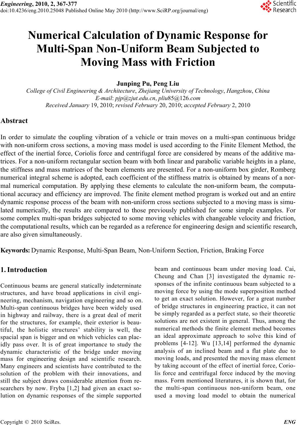Engineering, 2010, 2, 367-377
doi:10.4236/eng.2010.25048 Published Online May 2010 (http://www.SciRP.org/journal/eng)
367
Numerical Calculation of Dynamic Response for
Multi-Span Non-Uniform Beam Subjected to
Moving Mass with Friction
Junping Pu, Peng Liu
College of Civil Engineering & Architecture, Zhejiang University of Technology, Hangzhou, China
Received January 19, 2010; revised February 20, 2010; accepted February 2, 2010
Abstract
In order to simulate the coupling vibration of a vehicle or train moves on a multi-span continuous bridge
with non-uniform cross sections, a moving mass model is used according to the Finite Element Method, the
effect of the inertial force, Coriolis force and centrifugal force are considered by means of the additive ma-
trices. For a non-uniform rectangular section beam with both linear and parabolic variable heights in a plane,
the stiffness and mass matrices of the beam elements are presented. For a non-uniform box girder, Romberg
numerical integral scheme is adopted, each coefficient of the stiffness matrix is obtained by means of a nor-
mal numerical computation. By applying these elements to calculate the non-uniform beam, the computa-
tional accuracy and efficiency are improved. The finite element method program is worked out and an entire
dynamic response process of the beam with non-uniform cross sections subjected to a moving mass is simu-
lated numerically, the results are compared to those previously published for some simple examples. For
some complex multi-span bridges subjected to some moving vehicles with changeable velocity and friction,
the computational results, which can be regarded as a reference for engineering design and scientific research,
are also given simultaneously.
Keywords: Dynamic Response, Multi-Span Beam, Non-Uniform Section, Friction, Braking Force
1. Introduction
Continuous beams are general statically indeterminate
structures, and have broad applications in civil engi-
neering, mechanism, navigation engineering and so on.
Multi-span continuous bridges have been widely used
in highway and railway, there is a great deal of merit
for the structures, for example, their exterior is beau-
tiful, the holistic structures’ stability is well, the
spacial span is bigger and on which vehicles can plac-
idly pass over. It is of great importance to study the
dynamic characteristic of the bridge under moving
mass for engineering design and scientific research.
Many engineers and scientists have contributed to the
solution of the problem with their innovations, and
still the subject draws considerable attention from re-
searchers by now. Fryba [1,2] had given an exact so-
lution on dynamic responses of the simple supported
beam and continuous beam under moving load. Cai,
Cheung and Chan [3] investigated the dynamic re-
sponses of the infinite continuous beam subjected to a
moving force by using the mode superposition method
to get an exact solution. However, for a great number
of bridge structures in engineering practice, it can not
be simply regarded as a perfect state, so their theoretic
solutions are not existent in general. Thus, among the
numerical methods the finite element method becomes
an ideal approximate approach to solve this kind of
problems [4-12]. Wu [13,14] performed the dynamic
analysis of an inclined beam and a flat plate due to
moving loads, and presented the moving mass element
by taking account of the effect of inertial force, Corio-
lis force and centrifugal force induced by the moving
mass. Form mentioned literatures, it is shown that, for
the multi-span continuous non-uniform beam, one
used a moving load model to obtain the numerical

J. P. PU ET AL. 368
results in general, but did not consider the effect of
inertial force, Coriolis force and centrifugal force.
Some numerical examples dealt with above effect but
just analyzed the simple uniform beam. This paper has
been performed some complex problems (include
multi-span non-uniform beam with moving mass). For
a non-uniform rectangular section beam with both linear
and parabolic variable heights in a plane, the stiffness
and mass matrices of the beam elements have been de-
ducted. For a non-uniform box girder which can be
widely used in engineering structures, since the integral
formula of stiffness matrix is extremely complex, it is
difficult to write down the expression of the stiffness
coefficients, so Romberg numerical integral scheme is
adopted. Each coefficient of the stiffness matrix can
be obtained by means of a normal numerical computa-
tion. For some complex multi-span bridges subjected
to some moving vehicles with changeable velocities
and frictions, numerical results of dynamic responses
are also obtained, which can be regarded as a reference
for engineering design and scientific research.
2. Forced Vibration Differential Equation of
Euler-Bernoulli Beam
Forced vibration differential equation of Euler-Bernoulli
beam in plane bending with damping takes the form
),()()(
)()(
2
2
2
3
2
2
2
2
2
2
txf
t
y
xc
t
y
xm
xt
y
xI
x
c
x
y
xEI
xs
































(1)
where, the mass per unit length of the beam is m(x) = ρA,
while ρ is the material density and A is the area of the
cross section of the beam, c
s is damping coefficient of
strain rate, c(x) is damping coefficient of displacement
rate.
When a concentrate excited force P(t) was exerted at xi
＝vt of the beam, the force can be expressed, by using
the Dirac Delta function δ, as
(,) ()()
i
f
xtPtxvt


(2)
where v is the moving velocity. When a moving mass M
with the constant velocity moved on the beam, the action
force on the beam can be considered as a common effect
of the gravity and inertia force according to reference
literature [15].
)()],([),(vtxtvtygMtxf 

 (3)
Thus the formula (1) will be a set of systems of second
order differential equations with time-variant coefficient,
it needs to be solved by means of numerical method.
Lee’s investigation indicated, in literature [16,17], that
when the moving mass M with the constant velocity
moved on the Euler-Bernoulli beam, including the grav-
ity and inertia force induced by moving mass M, one still
needs to consider the effect of Coriolis force and cen-
trifugal force on the beam, that is
)()],(
),(2),([),(
2vtxtvtyv
tvtyvtvtygMtxf








 (4)
Considering the contact friction between the wheels
and the beam, a axial force X(ξ,t) should be exerted on
the beam, thus the action force on the beam can be ex-
pressed as follows
)(
),()],(
),(2),([
),( 2 














x
tXtyv
tyvtygM
txf
 (5)
When a moving vehicle has a brake on the bridge at a
moment tn, if the contact friction is big enough, the vehi-
cle will stop at moment tn+1, the axial force X(ξ,t) can be
expressed as
0
),( MatX



, (6)
)0( n tt 
)(),( 0 agMtX




, (7)
)(1  nn ttt
0),(

tX

. (8)
)( 1 n tt
where a0 is the initial acceleration of the vehicle, μ and g
represent the friction factor and that of gravity, respec-
tively. If the moving vehicle does not brake on the bridge
at any moment, the axial force X(ξ,t) will be expressed as
0
),( MatX



(9)
)0(t
The position ξ of the moving vehicle at the bridge can
be expressed as follows (see Figure 1)
2
000 5.0 tatvx 

, (10)
)( n tt
2
)(5.0)( nnnnn ttattvx  
)(1

nn ttt (11)
nnn avx2/
2
 
. (12)
)( 1 n tt
where v0 is the initial velocity, the position, velocity and
acceleration at moment tn are, respectively,
2
000 5.0 nnn tatvxx  , (13)
nn tavv 00 

, (14)
gaan



0. (15)
3. Discrete Model of Vibration Equations
under Moving Mass
According to the finite element method, the forced
vibration differential equation of Euler-Bernoulli beam
in plane bending with damping can be written, in matrix
form, as follows
)()()()( tttt FKyyCyM 

 (16)
where
),(),(),()( tttt av



XPPF


(17)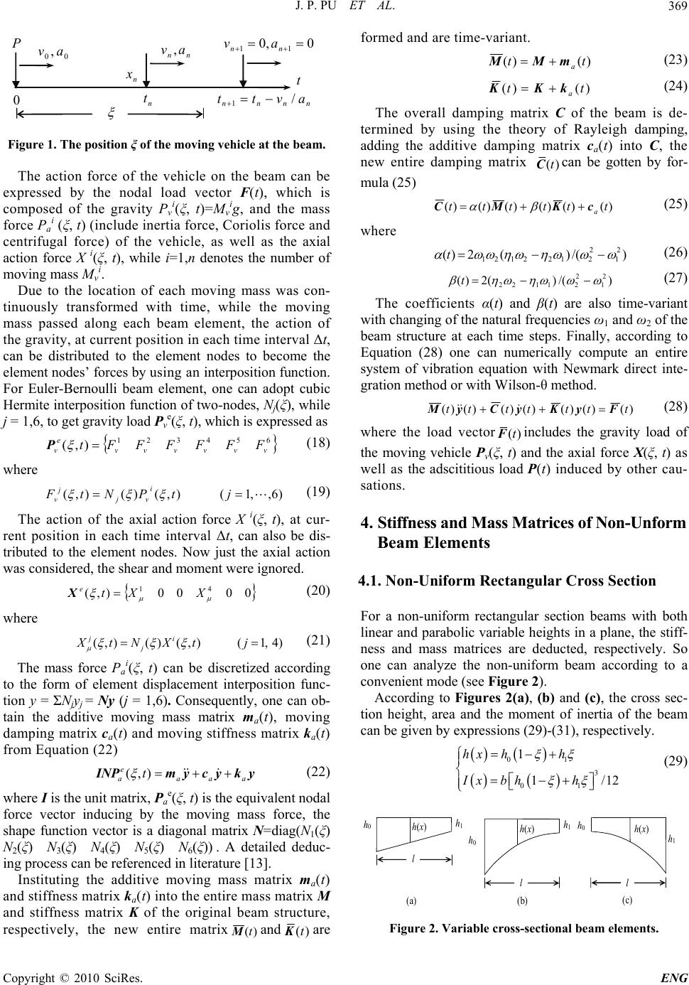

J. P. PU ET AL.369
n
t
t
n
x
P
00 ,av nn av,
0
0,0 11

 nnav

nnnn avtt/ 1 
Figure 1. The position ξ of the moving vehicle at the beam.
The action force of the vehicle on the beam can be
expressed by the nodal load vector F(t), which is
composed of the gravity Pv
i(ξ, t)=Mv ig, and the mass
force Pa
i (ξ, t) (include inertia force, Coriolis force and
centrifugal force) of the vehicle, as well as the axial
action force X i(ξ, t), while i=1,n denotes the number of
moving mass Mv
i.
Due to the location of each moving mass was con-
tinuously transformed with time, while the moving
mass passed along each beam element, the action of
the gravity, at current position in each time interval Δt,
can be distributed to the element nodes to become the
element nodes’ forces by using an interposition function.
For Euler-Bernoulli beam element, one can adopt cubic
Hermite interposition function of two-nodes, Nj(ξ), while
j = 1,6, to get gravity load Pv
e(ξ, t), which is expressed as


654321
),( vvvvvv
e
vFFFFFFt 
 P (18)
where
)6,,1(),()(),(  jtPNtF i
vj
j
v

(19)
The action of the axial action force X i(ξ, t), at cur-
rent position in each time interval Δt, can also be dis-
tributed to the element nodes. Now just the axial action
was considered, the shear and moment were ignored.


0000),(41

 XXt
eX (20)
where
(,)() (,)(1,4)
ji
j
XtNXtj

 
(21)
The mass force Pa
i(ξ, t) can be discretized according
to the form of element displacement interposition func-
tion y = ΣNjyj= Ny (j = 1,6). Consequently, one can ob-
tain the additive moving mass matrix ma(t), moving
damping matrix ca(t) and moving stiffness matrix ka(t)
from Equation (22)
ykycymINP aaa
e
at 
),( 
(22)
where I is the unit matrix, Pa
e(ξ, t) is the equivalent nodal
force vector inducing by the moving mass force, the
shape function vector is a diagonal matrix N=diag(N1(ξ)
N2(ξ) N3(ξ) N4(ξ) N5(ξ) N6(ξ)) . A detailed deduc-
ing process can be referenced in literature [13].
Instituting the additive moving mass matrix m
a(t)
and stiffness matrix ka(t) into the entire mass matrix M
and stiffness matrix K of the original beam structure,
respectively, the new entire matrix)(tMand ()t
K
are
formed and are time-variant.
)()( tt a mMM  (23)
() ()
a
tKKkt
(24)
The overall damping matrix C of the beam is de-
termined by using the theory of Rayleigh damping,
adding the additive damping matrix ca(t) into C, the
new entire damping matrix ()tCcan be gotten by for-
mula (25)
)()()()()()( tttttt a cKMC  
(25)
where
)/()(2)( 2
1
2
2122121
 t (26)
)/()(2)(2
1
2
21122
 t (27)
The coefficients α(t) and β(t) are also time-variant
with changing of the natural frequencies ω1 and ω2 of the
beam structure at each time steps. Finally, according to
Equation (28) one can numerically compute an entire
system of vibration equation with Newmark direct inte-
gration method or with Wilson-θ method.
)()()()()()()( ttttttt FyKyCyM   (28)
where the load vector()t
F
includes the gravity load of
the moving vehicle Pv(ξ, t) and the axial force X(ξ, t) as
well as the adscititious load P(t) induced by other cau-
sations.
4. Stiffness and Mass Matrices of Non-Unform
Beam Elements
4.1. Non-Uniform Rectangular Cross Section
For a non-uniform rectangular section beams with both
linear and parabolic variable heights in a plane, the stiff-
ness and mass matrices are deducted, respectively. So
one can analyze the non-uniform beam according to a
convenient mode (see Figure 2).
According to Figures 2(a), (b) and (c), the cross sec-
tion height, area and the moment of inertia of the beam
can be given by expressions (29)-(31), respectively.




 
01
3
01
1
1/
hx hh
Ix bhh







12
(29)
h
0
h
1
h(x)
l
h
0
h
1
h(x)
l
h
0
h
1
h(x)
l
(a) (b) (c)
Figure 2. Variable cross-sectional beam elements.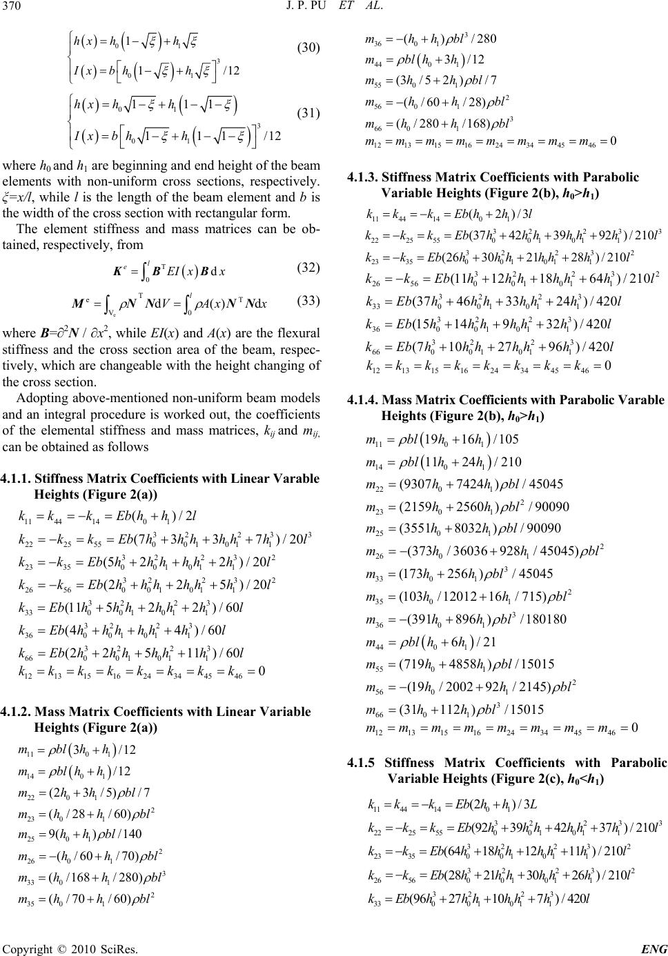

J. P. PU ET AL. 370




01
3
01
1
1/
hx hh
Ix bhh







12
(30)




01
3
01
111
111
hx hh
Ix bhh







/12
3
l
(31)
where h0 and h1 are beginning and end height of the beam
elements with non-uniform cross sections, respectively.
ξ=x/l, while l is the length of the beam element and b is
the width of the cross section with rectangular form.
The element stiffness and mass matrices can be ob-
tained, respectively, from

T
0d
l
eEI xx
KB B
(32)
  lxxAV 0
T
T
V
ed)(d
e
NNNNM 
(33)
where B=∂2N / ∂x2, while EI(x) and A(x) are the flexural
stiffness and the cross section area of the beam, respec-
tively, which are changeable with the height changing of
the cross section.
Adopting above-mentioned non-uniform beam models
and an integral procedure is worked out, the coefficients
of the elemental stiffness and mass matrices, k
ij and mij,
can be obtained as follows
4.1.1. Stiffness Matrix Coefficients with Linear Varable
Heights (Figure 2(a))
1144140 1
32 23
222555001011
32232
2335001011
32232
26560010 11
32 23
330010 11
3
360 0
()/2
(7337) / 20
(522) /20
(225)/ 20
(11522)/ 60
(4
kk kEbhhl
kkkEbhhhhhh
kkEbhhhhhhl
kkEbhhhhhhl
kEbhhhhh hl
kEbhh
 
 
 
 


223
101 1
322 3
66001011
12131516 2434 45 46
4)/60
(22511) / 60
0
hhh hl
kEbhhhhh hl
kkkkkkkk



4.1.2. Mass Matrix Coefficients with Linear Variable
Heights (Figure 2(a))


110 1
1401
220 1
2
23 01
250 1
2
26 01
3
33 01
2
35 01
3/12
/12
(23/ 5)/ 7
(/28/60)
9() /140
(/ 60/ 70)
(/168/ 280)
(/ 70/ 60)
mblhh
mblhh
mhhbl
mh h bl
mhhbl
mhhbl
mh hbl
mhhbl













 



3
360 1
4401
55
()/280
3/12
(3
m hhbl
mblhh
mh


 

01
2
56 01
3
66 01
12 13 15 1624344546
/52 )/7
(/60/28)
(/ 280/168)
0
hbl
mh h bl
mhh bl
mmmmmmmm




 



4.1.3. Stiffness Matrix Coefficients with Parabolic
Variable Heights (Figure 2(b), h0>h1)
11 441401
32 23
2225550010 11
3223 2
23350010 11
(2)/3
(37423992) / 210
(26302128) /210
kkkEbh hl
kkkEbh hhhh h
kkEbhhhhhh l
 
 
 
3
l
2
l
3223
26560010 11
32 23
33001011
322 3
360010 11
322 3
660010 11
12131516 24 34 4546
(11121864) / 210
(37463324) /420
(1514932) / 420
(7102796) /420
0
kkEbhhhhhh
kEbhhh hhhl
kEbh hhhhhl
kEbh hh hhhl
kkkkkkkk
 




4.1.4. Mass Matrix Coefficients with Parabolic Varable
Heights (Figure 2(b), h0>h1)



1101
140 1
220 1
2
230 1
250 1
2
26 01
3
3301
35 0
1916/105
1124/ 210
(93077424)/ 45045
(21592560)/ 90090
(35518032)/ 90090
(373/36036928/45045)
(173256)/ 45045
(103/ 120
mblhh
mblhh
mhhbl
mhhbl
mhhbl
mhhbl
mhhbl
mh












 



2
1
3
360 1
4401
55 0 1
2
56 01
3
660 1
12131516 24 34 45 46
1216/ 715)
(391896 )/180180
6/21
(7194858 )/15015
(19/ 200292/ 2145)
(31112 )/15015
0
hbl
mhhbl
mblhh
mhhbl
mhh bl
mhhbl
mmmmmmmm







 


 



4.1.5 Stiffness Matrix Coefficients with Parabolic
Variable Heights (Figure 2(c), h0<h1)
11441401
32 23
2225550010 11
3223 2
23350010 11
32232
2656001011
322
330010 11
(2)/ 3
(92394237) / 210
(64181211)/ 210
(28213026) / 210
(96 27107
kk kEbhhL
kkkEbhhhhhh
kkEbhhhhhhl
kkEbhhhhhh l
kEbhhh hhh

 
 
 

3)/420l
3
l

J. P. PU ET AL.371
l
322 3
36001011
32 23
66001011
12131516 24 34 4546
(3291415) /420
(24334637)/ 420
0
kEbhhh hhhl
kEbhhhhhh
kkkkkkkk



4.1.6. Mass Matrix Coefficients with Parabolic Varable
Heights (Figure 2(c), h0<h1)



110 1
140 1
220 1
2
23 01
2501
2
26 01
3
330 1
35 01
6/21
2411/ 210
(4858719 )/15015
(92/ 214519/ 2002)
(80323551)/ 90090
(16/ 715103/12012)
(11231 )/15015
(928/ 45045373/
mblhh
mblhh
mhhbl
mhh bl
mhhbl
mhh bl
mhhbl
mhh












 



2
3
360 1
440 1
36036)
(896391)/180180
1619 /105
bl
mhhbl
mblhh



 

550 1
2
560 1
3
6601
12 13 151624344546
(74249037)/45045
(25602159)/ 90090
(256173)/ 45045
0
mhhbl
mhhbl
mhhbl
mmmmmmmm




 


4.2. Non-Uniform Box Girder Section
The box section is shown in Figure 3 with an up bottom
width of B and a down bottom width of D. The thick-
nesses of both up and down bottom board are T. The
ventral shield thickness is C, and the section height of the
box girder is h(x). The centroid distance w from cen-
troidal axis z to z′ axis of self-defined is
2
() (2)() 0.5()
2()( 4)
() ChxDCThxBD T
ChxBDCT
wx  

2 (34)
So the area and moment of inertia can be denoted by a
section height h(x) and a centroid distance w(x) as fol-
lows
()2()(4 )
A
xChxBDCT (35)


2
3
2
33
2
() 2
1
() ()
6
()
2()()
2
11
(2)
12 12
(2)() ()
2
T
BTw x
IxChx T
hxT
ChxTwx
BTDCT
T
DCThxwx





 



 



 



(36)
Hypothesis that using a linear and parabolic variable
mode such as Figure 2, the beam height h(x) of box
girder element can also be denoted by formula 29, 30 and
31. Since w(x) is a composite function of h(x), so the
moment of inertia I(x) is also a very complex composite
function, moreover have some rational fractions in it. It
is difficult to get a fixed form integral result by a manual
calculation, so Romberg numerical integral scheme is
adopted in this paper. The numerical integral precision is
controlled to be 10-6. Each coefficient of the stiffness
matrix of non-uniform section box girder element can be
obtained by means of Formula (37).
2
2
22
0
()
()
()
lj
i
ij
dN x
dN x
kEIx
dx dx







dx


(37)
When deducing the mass matrix of non-uniform sec-
tion box girder element, since the area function A(x) is
relatively simple, so we adopt a manual calculation
fashion and the fixed form integral result is gotten. Ob-
serving Formula (35), and comparing the area formula of
a rectangular cross section, a superfluous item (B+D-4C)
T is found. These coefficients are constants. Form the
general Expressions (33) of mass matrix, it is easily
known that the mass matrix of non-uniform section box
girder element is gotten, as long as substituting the pa-
rameter b into 2C and adding an item (such as Formula
(38)) in mass matrix of rectangular cross section beam
element.
0
(4)
lT
e
M
BD CTNNdx 

 
  (38)
For referring and using conveniently, based on be-
fore-mentioned three non-uniform section modes, the
deduced results for all elements mij of mass matrix of box
girder element are enumerated as follows.
4.2.1. Mass Matrix Coefficients of the Box Girder with
Linear Variable Heights (Figure 2(a))





 
 
 


1101
1401
440 1
220 1
2
230 1
250 1
2
2601
32 4/6
4/6
32 4/6
210 3134/35
157114/210
94
276 13
mlChhTBDC
mlChhTBDC
mlChhTBDC
mlChh TBDC
mlChhTBDC
mlChhTBDC
mlChhTB



























 

 
3
3301
2
350 1
3
360 1
4/42
53 44/420
26 7134 /420
4/140
DC
mlChhTBDC
mlChhTBDC
mlChhTBDC















/70
0

J. P. PU ET AL. 372
C
D
B
h(x) T
T
z
y
z’
w
Figure 3. Geometry size of cross section of the box girder.
 

 
55 0
2
560 1
3
660 1
12 13 15 1624 344546
2310134/35
715114/ 210
3544/ 420
0
mlChhTBDC
mlChhTBDC
mlChhTBDC
mmmmmmmm













4.2.2. Mass Matrix Coefficients of the Box Girder with
Parabolic Variable Heights (Figure 2(b), h0>h1)








110 1
140 1
4401
220 1
2
230 1
25
2 1916354/105
21124354/ 210
267 4/21
293077424167314/45045
22159256047194/ 90090
2 3551
mlChh TBDC
mlChh TBDC
mlChhTBDC
mlC hhTBDC
mlC hhTBDC
mlC












 













01
2
260 1
3
330 1
2
350 1
3
3601
8032115834/ 90090
21865 371255774 /180180
21732564294/ 45045
2 1545403255774/180180
2391 89612874
hh TBDC
mlC hhTBDC
mlCh hTBDC
mlC hhTBDC
mlC hhTBDC





 


 













55 0
2
560 1
3
660 1
1213151624 34 45 46
/180180
2 719485855774/15015
2855386447194/ 90090
2 311121434/15015
0
mlCh h TBDC
mlC hhTBDC
mlCh hTBDC
mmmmmmmm








 




 










4.2.3 Mass Matrix Coefficients of the Box Girder with
Parabolic Variable Heights (Figure 2(c), h0<h1)








220 1
2
230 1
25 0
110 1
1401
440 1
2/21
/210
/105
2 485871955774/15015
2128828515734/ 30030
2 8032
67 4
22411354
216 19354
C
mlC hhTBDC
mlC hhTBDC
mlCh
ml hhTBDC
mlChhTBDC
mlChhTBDC





















1
3551115834/ 90090hTBDC






 
 

2
260 1
3
3301
1
350 1
360 1
55 0
2
3
2134451518594/ 60060
2 11203114304/150150
3712 1865/180180
896 /180180
2 74249037
255774
2391 12874
16
mlCh hTBDC
mlC hhTBDC
C
mlC hhTBDC
mlC hhTBDC
mlh h





 








 




 
2
560 1
3
660 1
121315162434 45 46
/ 45045
225602159/ 90090
2256173/ 45045
0
731 4
4719 4
429 4
C
C
TB DC
mlh hTBDC
mlh hTBDC
mmmmmmmm








 

 

4.2.3 Mass Matrix Coefficients of the Box Girder with
Parabolic Variable Heights (Fig. 2(c), h0<h1)








1101
140 1
440 1
220 1
2
230 1
25 0
2674 /21
22411354/210
2 1619354/105
2 485871955774/15015
2128828515734/ 30030
2 8032
mlChhTBDC
mlChhTBDC
mlChhTBDC
mlC hhTBDC
mlChhTBDC
mlCh

















 







1
2
260 1
3
330 1
2
350 1
3
360 1
3551115834/ 90090
2 1344 51518594 /60060
2 11203114304/150150
2 3712186555774/180180
2 896 39112874 /1
hTBDC
mlCh hTBDC
mlC hhTBDC
mlChhTBDC
mlC h hTBDC




 














550 1
2
560 1
3
660 1
12 13 15 1624 3445 46
80180
274249037167314/45045
22560215947194/90090
22561734294/45045
0
mlC hhTBDC
mlChhTBDC
mlChhTBDC
mmmmmm mm







 





h
0
h
1 h
0
5. Numerical Examples
5.1. Validation
In order to demonstrate the feasibility of the present
stiffness and mass element matrices, a simple example is
performed, that is, a non-uniform cross section beam
with the length l = 20 m, the width of the rectangular
section is b = 0.2 m, the small end and the big end height
are h1 = 0.1 m and h0= 0.3 m, respectively. Young’s
modulus is E = 3.0 × 1010 N/m2, the concentrate load is F
= 10 kN, the shape of the beam is shown in Figure 4.
l
F
Figure 4. Shape of the beam.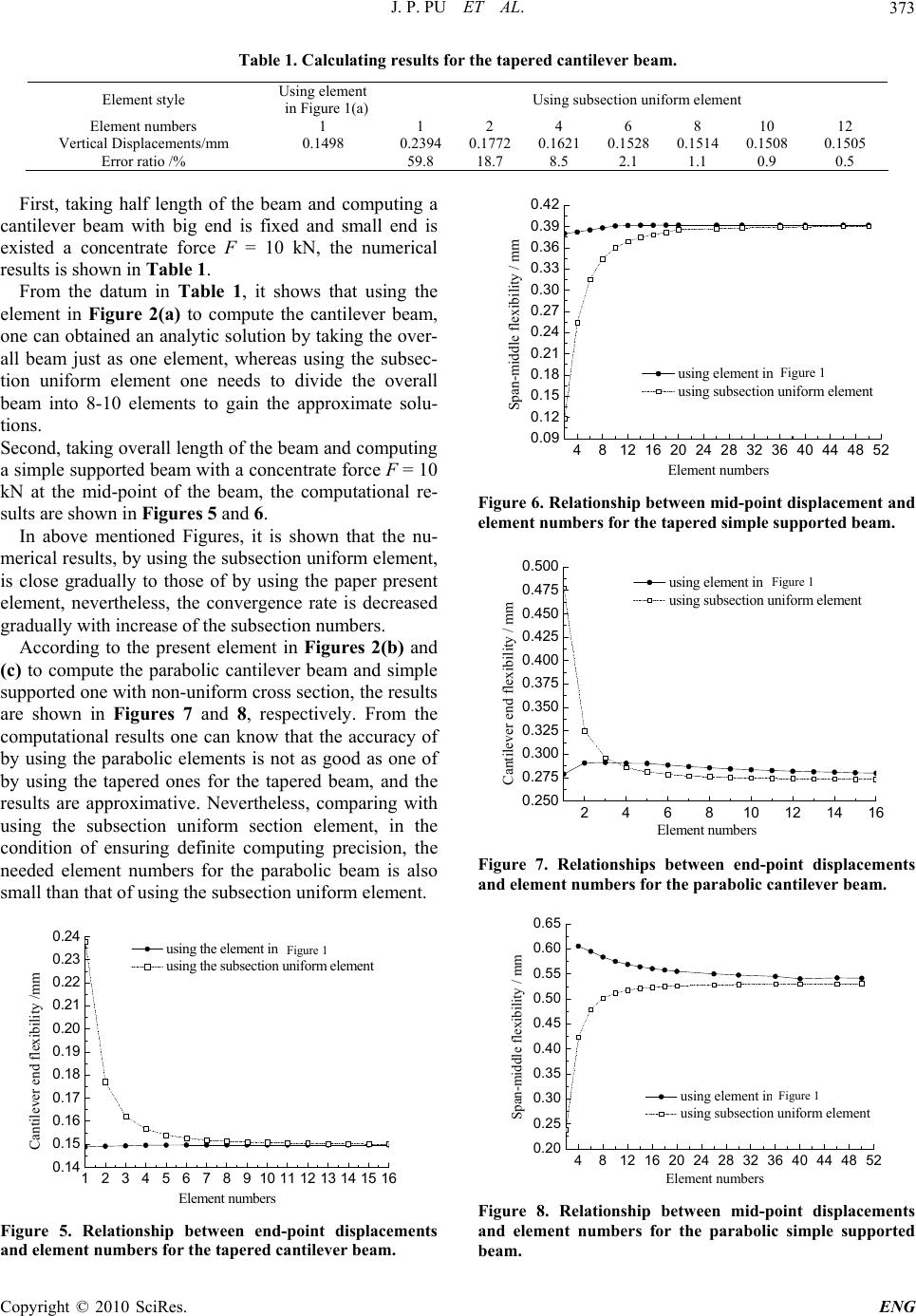

J. P. PU ET AL. 373
Table 1. Calculating results for the tapered cantilever beam.
Element style Using element
in Figure 1(a) Using subsection uniform element
Element numbers 1 1 2 4 6 8 10 12
Vertical Displacements/mm 0.1498 0.23940.17720.16210.15280.1514 0.1508 0.1505
Error ratio /% 59.8 18.7 8.5 2.1 1.1 0.9 0.5
First, taking half length of the beam and computing a
cantilever beam with big end is fixed and small end is
existed a concentrate force F = 10 kN, the numerical
results is shown in Table 1.
4812 16 20 24 28 32 36 40 44 48 52
0.09
0.12
0.15
0.18
0.21
0.24
0.27
0.30
0.33
0.36
0.39
0.42
Span-middle flexibility / mm
Element numbers
using element in Fig.1
using subsection uniform element
Figure 1
From the datum in Table 1, it shows that using the
element in Figure 2(a) to compute the cantilever beam,
one can obtained an analytic solution by taking the over-
all beam just as one element, whereas using the subsec-
tion uniform element one needs to divide the overall
beam into 8-10 elements to gain the approximate solu-
tions.
Second, taking overall length of the beam and computing
a simple supported beam with a concentrate force F = 10
kN at the mid-point of the beam, the computational re-
sults are shown in Figures 5 and 6. Figure 6. Relationship between mid-point displacement and
element numbers for the tapered simple supported beam.
In above mentioned Figures, it is shown that the nu-
merical results, by using the subsection uniform element,
is close gradually to those of by using the paper present
element, nevertheless, the convergence rate is decreased
gradually with increase of the subsection numbers.
246810 12 1416
0.250
0.275
0.300
0.325
0.350
0.375
0.400
0.425
0.450
0.475
0.500
Cantilever end flexibility / mm
Element numbers
using element in Fig.1
using subsection uniform element
Figure 1
According to the present element in Figures 2(b) and
(c) to compute the parabolic cantilever beam and simple
supported one with non-uniform cross section, the results
are shown in Figures 7 and 8, respectively. From the
computational results one can know that the accuracy of
by using the parabolic elements is not as good as one of
by using the tapered ones for the tapered beam, and the
results are approximative. Nevertheless, comparing with
using the subsection uniform section element, in the
condition of ensuring definite computing precision, the
needed element numbers for the parabolic beam is also
small than that of using the subsection uniform element.
Figure 7. Relationships between end-point displacements
and element numbers for the parabolic cantilever beam.
4812 1620 24 28 3236 40 4448 52
0.20
0.25
0.30
0.35
0.40
0.45
0.50
0.55
0.60
0.65
Span-middle flexibility / mm
Element numbers
using element in Fig.1
using subsection uniform element
Figure 1
12345678910111213141516
0.14
0.15
0.16
0.17
0.18
0.19
0.20
0.21
0.22
0.23
0.24
Cantilever end flexibility /mm
Element numbers
using the element in Fig.1
using the subsection uniform element
Figure 1
Figure 8. Relationship between mid-point displacements
and element numbers for the parabolic simple supported
beam.
Figure 5. Relationship between end-point displacements
and element numbers for the tapered cantilever beam.

J. P. PU ET AL. 374
By applying the present element to analyze the non-
uniform rectangular beams with both linear and parabolic
variable heights, the results are being approached the
accurate solutions much more. A non- uniform cantilever
beam element and a non-uniform simple supported beam
are presented to validate the element’s reliability, and the
calculating results shows that, if using the subsection
uniform finite elements one needs to divide more ele-
ments to converge the numerical solution to the current
exact solution. Therefore, by applying the present ele-
ment to analysis the non-uniform beam, the analysis can
be simplified distinctly and the computational results will
approach the accurate solutions.
5.2. A Three-Span Continuous Haunched Bridge
under a Moving Load
In this example a three-span non-uniform continuous
bridge is performed, the height of the beam is changeable
in the plane (see Figure 9). A single load value of Pv=
100 kN, moving at a speed of v ＝ 17 m/s, is considered.
Total length of the bridge is L = 60 m, Young’s modulus is
E = 3 × 1010 N/m2 and the mass density is ρ ＝ 2400 kg/m3.
The acceleration of the gravity is g = 9.81m/s2 in all ex-
amples. The damping coefficient is ζ1 = ζ2 = 0.005 and
the associated natural frequencies are ω1 and ω2, which
were obtained in the main dynamic program.
First, a case of which the haunched bridge with damp-
ing subjected to a moving load, is considered. In this
case the natural frequencies are not time-variant, because
in this example the effects of inertial force, Coriolis force
and centrifugal force induced by the moving mass have
been ignored, so the mass, stiffness and damping matri-
ces of the entire vibrating system are not time-variant yet.
The finite element model of the bridge is composed of 36
uniform beam elements and 24 tapered beam elements.
The numerical results for the deflections at each mid-
span position are in excellent agreement with those
available ones from the reference literature [6,8].
Next considering the bridge with damping subjected to
a moving mass, since the effect of the inertial force,
Coriolis force and centrifugal force induced by the mov-
ing mass is existent, the overall matrices(include mass,
stiffness and damping) and the associated natural fre-
quencies are all time-variant at each computing time
1.0-1.6 m
1.0 m
1.6 m
0.5 m
A
A
v
P= 100 kN
12 m 6 m 6 m12 m
6 m 6 m
12 m
Span-1 Span-3
Figure 9. A three-span continuous haunched bridge under a
moving load.
step. The numerical results for the deflections at each
mid-span position of the bridge are shown in Figure 10.
From Figure 10 it is shown that the difference of the
displacements, for the case with moving load and with
moving mass, is no evident. Since the deflections of the
bridge are small, the effects of inertial force, Coriolis
force and centrifugal force induced by the moving mass
are also small to the dynamical responses of the bridge.
Nevertheless, the last effect may be significant for other
cases.
5.3. A Simple Supported Beam under a Moving
Mass with Uniform Variable Speeds
Considering a simple supported beam under a moving
mass with uniform variable speeds (see Figure 11), the
length of the beam is L = 100 m, Young’s modulus is E =
2.15 × 1011 Pa, the mass density of the beam is ρ = 6375
kg/m3 and the section area is A = 2.4 m2, the moment of
inertia is I = 0.8 m4, the moving mass mv = 61.2 × 103 kg.
We divided the beam into 50 beam elements, and
taken the time step as Δt = 0.02 s, the initial velocity of
the moving mass is v = 20 m/s, and the acceleration are a
= 0, ±3, ±6 and ±9 m/s2, respectively. The dynamical
displacement results of the mid-point of the beam have
been computed by adopting the Newmark method. Under
the conditions of being different accelerations (acceler-
ating and decelerating), the dynamical displacement
0.0 0.10.2 0.3 0.4 0.50.60.70.80.91.0
-0.004
-0.002
0.000
0.002
0.004
0.006
0.008
0.010
Displacement / m
x / L
ML(S-2) MM(S-2)
ML(S-1) MM(S-1)
ML(S-3) MM(S-3)
ML-moving load; MM-moving mass; S-span
Figure 10. Deflections at each mid-point position for each
span under a moving load/mass.
10 0 m
vt
x
m
v
EI, ρA
y
v, a
Figure 11. Simple supported beam under a moving mass
with uniform variable speeds.

J. P. PU ET AL.375
response contrast curves of the midpoint of the beam are
given in Figures 12 and 13, respectively.
From Figures 12 and 13 it is shown that, under the
conditions of being same initial velocity, the dynamical
displacements of the midpoint of the beam induced by
moving mass with acceleration is bigger than that of with
uniform velocity, and the larger the acceleration, the
bigger the midpoint displacements of the beam. Whereas
the dynamical displacements of the midpoint of the beam
induced by moving mass with deceleration is smaller
than that of with uniform velocity, and the larger the ac-
celeration, the smaller the midpoint displacements of the
beam. It is just opposite to the state with accelerated mo-
tion. It is because the moving mass was exerted by a fric-
tion induced between the contact interfaces.
When the moving mass motion with acceleration, it is
given a friction, which is in line with the movement di-
rection, by the beam. At the same time, the beam is sub-
jected to a reaction force imposed by the moving mass.
This force can be regarded as an axial pressure acting on
the beam. This pressure will generate an additional
bending moment in the beam, so that the deflection of
the beam will be increased. On the contrary, when the
01234
0.00
0.02
0.04
0.06
0.08
0.10
Displacement / m
T
/ s
a=0 m
a=3 m
a=6 m
a=9 m
Figure 12. Mid-point displacement of the beam with effect
of acceleration.
01234
0.00
0.02
0.04
0.06
0.08
0.10
a= 0 m
a=-3 m
a=-6 m
a=-9 m
Displacement / m
T
/ s
Figure 13. Mid-point displacement of the beam with effect
of deceleration.
moving mass deceleration movement, the beam will be
subjected to an axial tension, and this tension will gener-
ate an additional bending moment within the beam to
reduce the deflection.
5.4. A Three-Span Continuous Box Girder Bridge
with Non-Uniform Section under a Moving
Vehicle with Friction
The purpose of this example is to compute a three-span
continuous box girder bridge with non-uniform sections
under a moving vehicle with friction, the bridge is com-
posed of 7 box girder segments, the height of the box-
section is changeable with both linear and parabolic
soffit shape in the plane (see Figure 14). The total length
of the bridge is L = 120m, the mass density is ρ ＝ 2400
kg/m3 and Young’s modulus is E = 3 × 1010 N/m2. The
acceleration of the gravity is g = 9.81m/s2, the moment
of inertia I(x) is changeable with the position x. There is
a vehicle at left end of the bridge, the weight of the vehi-
cle is P = 20.6 × 104 N (while the front-wheel and rear
wheel are P
1 = 8.0 × 103 N and P2 = 12.6 × 103 N, re-
spectively), the space between the wheels is 2.0 m, at the
time of t = 0 the front-wheel is just in the left end of
bridge, the vehicle travels at a speed of v ＝15 m/s.
When the vehicle moves forward 30 meters from the
left end of the bridge at a uniform velocity, then it is bro-
ken, so the velocity will be slowed down or stopped by
contact friction. In order to impose the braking force, a
ramp function is assumed (see Figure 15). This is based
on the test results on highway vehicles conduced by the
Transport and Road Research Laboratory [18]. The brak-
ing force increases linearly to a maximum Fb max = εP and
then stays constant until the vehicle either comes to a
stop or crosses the bridge span and is written as
P
1
v
P
2
10 m20 m 20 m10 m 20 m 20 m 20 m
0.2 m
1 m
2 m
1 m－1.8 m 0.1 m
0.1 m
0.2 m
Figure 14. A three-span continuous box girder bridge with
variable sections.

J. P. PU ET AL. 376
max
1
max 1
(),
(1 )()
,
n
bn
nn
b
bn
tt
Ft
tt
F
FT









tT
tt
(39)
where ε is the impact coefficient, P is the vehicle static
weight, tn is the moment of begin braking and T is the
moment of the braking force increases to the maximum
value of Fbmax in time interval tn ≤ t ≤ tn+1.
For this example, 60 linear and parabolic beam ele-
ments are divided in overall bridge, the time step is Δt ＝
0.02 s. We take the friction coefficients as μ = 0.1, 0.2, 0.3
and 0.4, respectively. Taking the impact coefficient ε = 0.2,
the numerical results for the midpoint deflections at
mid-span position of the bridge are shown in Figure 16.
Figure 16 shows that the dynamical displacements
were affected by friction together with the impact coeffi-
cient. The larger the friction coefficient, the larger the
maximum dynamical displacements. The larger the fric-
tion, the shorter the time of braking vehicle. In the condi-
tion of being same friction force. The larger the impact
coefficient, the bigger the dynamical displacements of
midpoint at the mid-span of bridge. It can be observed
from Figure 17 in evidence.
tt
n n+ 1
0.1
0.2
0.3
0.4
ε
(1-ε
4
)( t
n+1
－t
n
) t
T
/ s
Impact coefficients
Figure 15. Relationship of braking time vs. impact coeffi-
cient.
01234 567 8910
-0.002
0.000
0.002
0.004
0.006
0.008
0.010
Displacement / m
T / s
without friction
 =0.1
 =0.2
 =0.3
 =0.4
μ = 0.1
μ = 0.2
μ = 0.3
μ = 0.4
Figure 16. Deflections of mid-point position at mid span (ε =
0.2).
012345678910
-0.002
0.000
0.002
0.004
0.006
0.008
0.010
Displacement / m
T / s
without friction
 =0
 =0.1
 =0.2
 =0.3
ε = 0
ε = 0.2
ε = 0.3
ε = 0.4
Figure 17. Deflections of mid-point position at mid span (μ
= 0.2).
5. Concluding Remarks
Dynamical solutions of the multi-span non-uniform
beam with a moving vehicle can not be obtained by the
theoretical means, the mass of the vehicle can not just be
regarded as a simple moving load, the effect of inertial
force, Coriolis force and centrifugal force is needed to be
considered in general. The use of box beam bridge with
non-uniform cross section is fairly common in the engi-
neering. Numerical analysis for dynamic response of this
kind of beam is beneficial to understand the dynamic
characteristics of the bridge, to provide the scientific
basis for the safe use of the bridge, and provided with a
certain practical significance and application values. Us-
ing oblique-shaped and Hparabolic-shaped beam element
with non-uniform cross section Hcan improve the accu-
racy and efficiency in solving. To define the dynamic
response effect of the bridge caused by vehicle moving
with variable speed as well as the friction and braking
impact force on the bridge deck needs to considered the
relationships of various factors synthetically, and then to
find a design scheme closer to engineering practice com-
bined with the relevant scientific experiment.
6
. References
[1] L. Fryba, “Vibration of Solids and Structures under
Moving Loads,” Noordhoff International Publishing,
Groningen, 1972.
[2] L. Fryba, “Dynamic Behaviour of Bridges due to High-
Speed Trains,” In: R. Delgado, R. Calcada and A. Cam-
pos Eds., Workshop Bridges for High-Speed Railways,
Faculty of Engineering, University of Porto, Porto, 2004,
pp.137-158.
[3] C. W. Cai, Y. K. Cheung and H. C. Chan, “Dynamic
Responses of Infinite Continuous Beams Subjected to a
Moving Force－An Exact Method,” Journal of Sound
and Vibration, Vol. 123, 1988, pp. 461-472.
[4] J. S. Wu and C. W. Dai, “Dynamic Responses of Mul-

J. P. PU ET AL. 377
tispan Nonuniform Beam due to Moving Loads,” Journal
of Structural Engineering, Vol. 113, 1987, pp. 458-474.
[5] H. P. Lee, “Dynamic Responses of a Beam with Interme-
diate Point Constraints Subject to a Moving Load,” Jour-
nal of Sound and Vibration, Vol. 171, 1994, pp. 361-368.
[6] G. Michaltsos, D. Sophianopoulos and A. N. Kounadis,
“The Effect of a Moving Mass and other Parameters on
the Dynamic Response of a Simply Supported Beam,”
Journal of Sound and Vibration, Vol. 191, 1996, pp.
357-362.
[7] K. Henchi, M. Fafard, G. Dhatt and M. Talbot, “Dynamic
Behavior of Multi-Span Beams under Moving Loads,”
Journal of Sound and Vibration, Vol. 199, 1997, pp.
33-50.
[8] H. C. Kwon, M. C. Kim and I. W. Lee, “Vibration Con-
trol of Bridges under Moving Loads,” Computers &
Structures, Vol. 66, 1998, pp. 473-480.
[9] D. Y. Zheng, Y. K. Cheung, F. T. K. Au and Y. S. Cheng,
“Vibration of Multi-Span Non-Uniform Beams under
Moving Loads by Using Modified Beam Vibration Func-
tions,” Journal of Sound and Vibration, Vol. 212, 1998,
pp. 455-467.
[10] Y. A. Dugush, M. Eisenberger, “Vibrations of Non-
Uniform Continuous Beams under Moving Loads,”
Journal of Sound and Vibration, Vol. 254, 2002, pp.
911-926.
[11] A. Yavari, M. Nouri, M. Mofid, “Discrete Element Analysis
of Dynamic Response of Timoshenko Beams under Moving
Mass,” Advances in Engineering Software, Vol. 33, 2002, pp.
143-153.
[12] A. E. Martinez-Castro, P. Museros and A. Castillo-
Linares, “Semi-Analytic Solution in the Time Domain for
Non-Uniform Multi-Span Bernoulli-Euler Beams Trav-
ersed by Moving Loads,” Journal of Sound and Vibration,
Vol. 294, 2006, pp. 278-297.
[13] J. J. Wu, “Dynamic Analysis of an Inclined Beam due to
Moving Loads,” Journal of Sound and Vibration, Vol.
288, 2005, pp. 107-131.
[14] J. J. Wu, “Vibration Analyses of an Inclined Flate Sub-
jected to Moving Loads,” Journal of Sound and Vibration,
Vol. 299, 2007, pp. 373-387.
[15] E. Esmailzadeh and M. Ghorashi, “Vibration Analysis of
Beams Traversed by Uniform Partially Distributed Mov-
ing Massed,” Journal of Sound and Vibration, Vol. 184,
1995, pp. 9-17.
[16] U. Lee, “Separation between the Flexible Structure and
the Moving Mass Sliding on it,” Journal of Sound and
Vibration, Vol. 209, 1998, pp. 867-877.
[17] U. Lee, C. H. Pak and S. C. Hong, “Dynamics of Piping
System with Internal Unsteady Flow,” Journal of Sound
and Vibration, Vol. 180, 1995, pp. 297-311.
[18] S. S. Law and X. Q. Zhu, “Bridge Dynamic Responses
due to Road Surface Roughness and Braking of Vehicle,”
Journal of Sound and Vibration, Vol. 282, 2005, pp.
805-830.