Paper Menu >>
Journal Menu >>
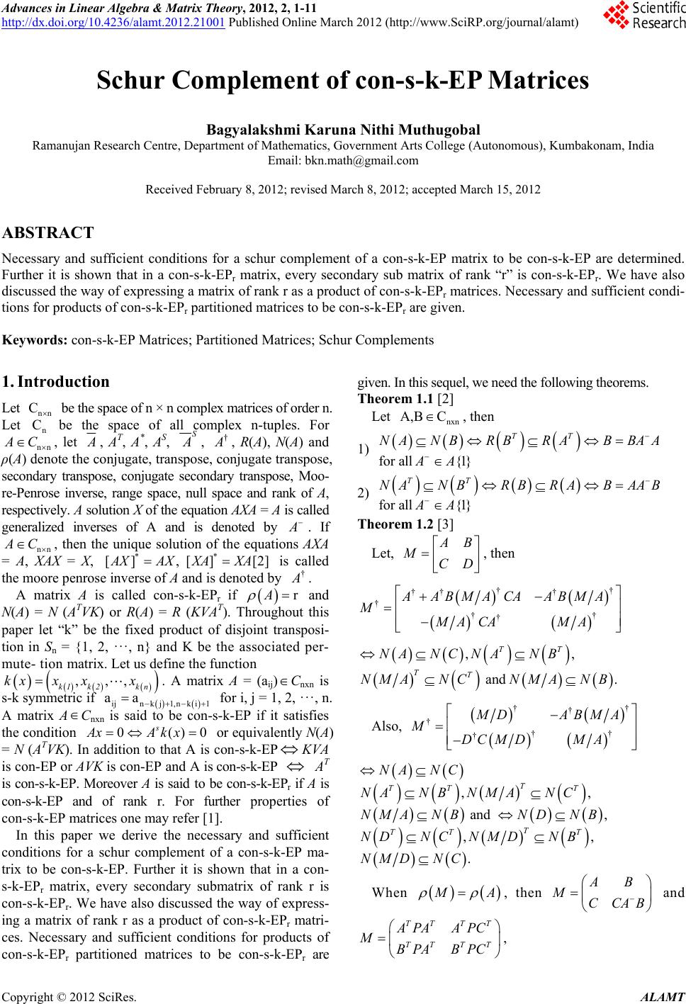 Advances in Linear Algebra & Matrix Theory, 2012, 2, 1-11 http://dx.doi.org/10.4236/alamt.2012.21001 Published Online March 2012 (http://www.SciRP.org/journal/alamt) Schur Complement of con-s-k-EP Matrices Bagyalakshmi Karuna Nithi Muthugobal Ramanujan Research Centre, Department of Mathematics, Government Arts College (Autonomous), Kumbakonam, India Email: bkn.math@gmail.com Received February 8, 2012; revised March 8, 2012; accepted March 15, 2012 ABSTRACT Necessary and sufficient conditions for a schur complement of a con-s-k-EP matrix to be con-s-k-EP are determined. Further it is shown that in a con-s-k-EPr matrix, every secondary sub matrix of rank “r” is con-s-k-EPr. We have also discussed the way of expr essing a matrix of r ank r as a produ ct of con- s-k-EP r matrices. Necessary and sufficient condi- tions for produ c t s of con -s- k-EPr partitioned matrices to be con-s-k-EPr are given. Keywords: con-s-k-EP Matrices; Partitioned Matrices; Schur Complements 1. Introduction Let be the space of n × n complex matrices of order n. Let be the space of all complex n-tuples. For nn nn C n C A C , let A , AT, A*, AS, S A, A †, R(A), N(A) and ρ(A) denote the conjugate, transpose, conjugate transpose, secondary transpose, conjugate secondary transpose, Moo- re-Penrose inverse, range space, null space and rank of A, respectively . A solution X of the equation AXA = A is called generalized inverses of A and is denoted by A . If nn A C , then the unique solution of the equations AXA = A, XAX = X, * [] , A XAX* [][2]XAXA is called the moore penrose inverse of A and is denoted by † A . A matrix A is called con-s-k-EPr if Ar and N(A) = N (ATVK) or R(A) = R (KVAT). Throughout this paper let “k” be the fixed product of disjoint transposi- tion in Sn = {1, 2, ···, n} and K be the associated per- mute- tion matrix . Let us define the function . A matrix A = (aij) ,,, k1 k2kn kxx xx Cnxn is s-k symmetric if ij nkj 1,nki 1 for i, j = 1, 2, · · · , n. A matrix ACnxn is said to be con-s-k-EP if it satisfies the condition or equivalently N(A) = N (ATVK). In addition to that A is con-s-k-EP aa 0 s AxA k ()x0 KVA is con-EP or AVK i s c o n - E P a n d A i s con-s-k-EP A T is con-s-k-EP. Moreover A is said to be con-s-k-EPr if A is con-s-k-EP and of rank r. For further properties of con-s-k-EP matrices one may ref er [1]. In this paper we derive the necessary and sufficient conditions for a schur complement of a con-s-k-EP ma- trix to be con-s-k-EP. Further it is shown that in a con- s-k-EPr matrix, every secondary submatrix of rank r is con-s-k-EPr. We have also discussed the way of express- ing a matrix of rank r as a product of con-s-k-EPr matri- ces. Necessary and sufficient conditions for products of con-s-k-EPr partitioned matrices to be con-s-k-EPr are given. In this sequel, we need the following theorems. Theorem 1.1 [2] Let nxn A,B C , then 1) for all {1} TT NANBRBRAB BAA AA 2) for all {1} TT NANBRBRAB AAB AA Theorem 1.2 [3] Let, A B MCD , then †† ††† † †† † AABMA CAABMA M MA CAMA ,, and . TT TT NANC NANB NMANCNMA NB Also, †† † † †† † MD ABMA M DC M DMA ,, and , ,, . T TT T T TT T NA NC NA NBNMA NC NMA NBNDNB ND NCNMD NB NMDNC When M A , then and AB MCCAB TTT T TTT T A PAA PC MBPA BPC , C opyright © 2012 SciRes. ALAMT 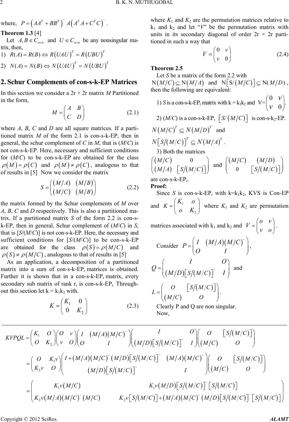 B. K. N. MUTHUGOBAL 2 where, TT TT P AABBAA ACC . Theorem 1.3 [4] Let ,nn A BC and nn UC be any nonsingular ma- trix, then, 1) () ()TT RA RBRUAURUBU TT 2) () ()NA NBNUAUNUBU 2. Schur Complements of con-s-k-EP Matrices In this section we consider a 2r × 2r matrix M Partitioned in the form, A B MCD (2.1) where A, B, C and D are all square matrices. If a parti- tioned matrix M of the form 2.1 is con-s-k-EP, then in general, the schur complement of C in M, that is (M/C) is not con-s-k-EP. Here, necessary and sufficient conditions for (M/C) to be con-s-k-EP are obtained for the class M C and M C , analogous to that of results in [5] . Now we consider the matrix M AMB S M CMB (2.2) the matrix formed by the Schur complements of M over A, B, C and D respectively. This is also a partitioned ma- trix. If a partitioned matrix S of the form 2.2 is con-s- k-EP, then in general, Schur complement of (M/C) in S, that is [S/(M/C)] is not con-s-k-EP. Here, the necessary and sufficient conditions for [S/(M/C)] to be con-s-k-EP are obtained for the class SM C and SM C , analogous to that of results in [5] As an application, a decomposition of a partitioned matrix into a sum of con-s-k-EPr matrices is obtained. Further it is shown that in a con-s-k-EPr matrix, every secondary sub matrix of rank r, is con-s-k-EPr. Through- out this section let k = k1k2 with. 1 2 0 0 K KK (2.3) where K1 and K2 are the permutation matrices relative to k1 and k2 and let “V” be the permutation matrix with units in its secondary diagonal of order 2r × 2r parti- tioned in such a way that 0 0 v v V (2.4) Theorem 2.5 Let S be a matrix of the form 2.2 with NN M CMA and N S/N( ) M CM D, then the following are equivalent: 1) S is a con-s-k-EPr matrix with k = k1k2 and V= 0 0 ν ν . 2) (M/C) is a con-s-k-EP, S/M C is con-s-k2-EP. TT M CMNND and TT SMC MANN . 3) Both the matrices 0MC MAS MC and 0 MC MD SMC are con-s-k-EPr. Proof: Since S is con-s-k-EPr with k=k1k2, KVS is Con-EP and where K1 and K2 are permutation matrices associated with k1 and k2 and . 1 2 KKo oK oν Vνo Consider IMAMC POI , SMC IO Q M DI and OSMC LMC O . Clearly P and Q are non singular. Now, 1 2 1 2 11 IO OSMC KO OνIMAMC KVPQL OK νOMDS MCIMCO OI IMAMCMDSMC MAMCOSMC OKν KνOMC O MDS MCI KνMC KνMDS MC 22 SMC KνMA MCMCKνSMCMAMC MDSMCSMC Copyright © 2012 SciRes. ALAMT 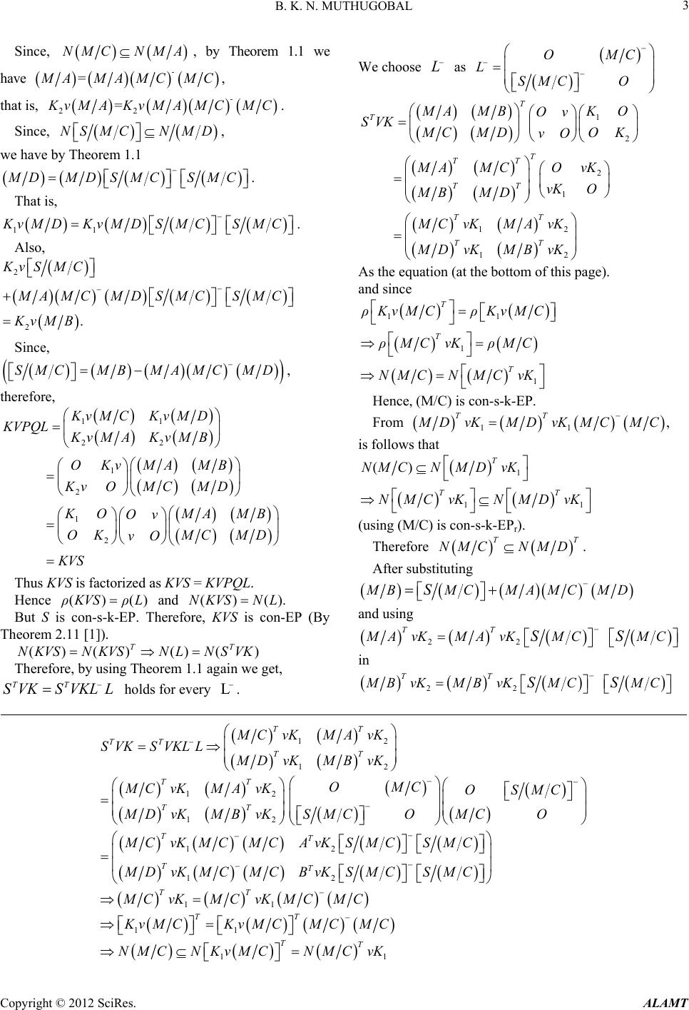 B. K. N. MUTHUGOBAL 3 Since, NMC NMA have , by Theorem 1.1 we - M A= MAM CM C, that is, 22 - KνMA=Kν M AMC MC. Since, NS MCN MD , we have by Theorem 1.1 M DMDSMC SMC . That is, 11 KνMD Kν M DSMCSMC . Also, 2 2. KνSMC M AMC MDSMCSMC KνMB Since, SMCMBMAMC MD , therefore, 11 22 1 2 1 2 KνMC KνMD KVPQL KνMA KνMB OKνMA MB KνOMCMD K OMAM Oν OKMCMD νO KVS B )). ) L as OMC L SMC O Thus KVS is factorized as KVS = KVPQL. Hence and ()(ρKVS ρL()(NKVS NL But S is con-s-k-EP. Therefore, KVS is con-EP (By Theorem 2.11 [1]). ()() ()( TT N KVSN KVSN LNS VK Therefore, by using Theorem 1.1 again we get, TT SVKSVKLL holds for every . L We choose 1 2 2 1 12 12 T T T TT TT TT TT M AMBKO Oν SVK M CMD OK νO MA MCOνK νKO MB MD MC νKMAνK MD νKMBνK As the equation (at the bottom of this page). and since 11 1 1 T T T ρKνMCρKν M C ρMC νKρMC NMCN MC νK Hence, (M/C) is con-s-k-EP. From 11 , TT MD νKMDν K MC MC is follows that 1 11 () T TT NMCN MD νK NMCνKNMDν K (using (M/C) is con-s-k-EPr). Therefore TT NMC NMD. After substituting M BMCMAMCMS D and using 22 TT MA νKMAν K MC MCSS in 22 TT MB νKMBνKMC MCSS 12 12 12 12 12 12 1 TT TT TT TT TT TT TT T MC νKMAνK SVK SVKLL MD νKMBνK OMC MC νKMAνKOSMC MC O SMC OMD νKMBνK MC νKMC MC AνKSMCSMC MD νKMCMC BνKSMCSMC MC νKMC 1 11 11 T TT TT νKMC MC KνMC KνMCMCMC NMC NKνMCNMC νK Copyright © 2012 SciRes. ALAMT 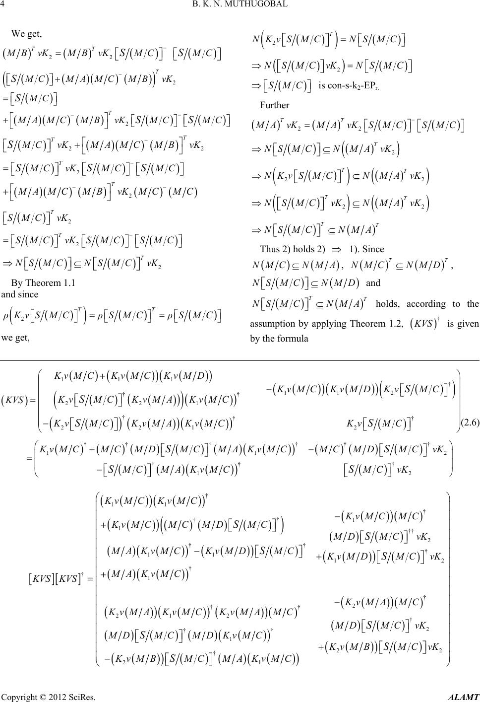 B. K. N. MUTHUGOBAL 4 We get, 22 TT MB νKMBν K MC MCSS 2 2 T T MCMAMCMBνK MC MA MCMBνKMCMC S S SS 22 2 2 T T T T MC νKMAMCMBν K MC νKMC MC MA MCMBνKMC MC S SSS 2 2 2 T T T SMC νK SMC ν K SMC SMC NS MCNSMCνK By Theorem 1.1 and since 2 TT ρKνSMC ρSMCρSMC we get, 2 T NKνSMC NSMC 2 NSMCν K NS MC SMC is con-s-k2-EPr. Further 22 2 22 22 TT T TT TT TT MA νKMAν K SMC SMC NS MCNMAνK NKνSMC NMAνK NSMCνKNMAνK NS MCNMA Thus 2) holds 2) 1). Since NMC NMA, TT NMC NMD, NS MCNMD and TT NS MCNMA holds, according to the assumption by applying Theorem 1.2, † K VS is given by the formula 111 † 11 2 †† 221 †† † 221 2 † † † †† † 112 † † † 1 2 KνMC KνMCKνMD KνMC KνMD KνMC KνMCKνMA KνMC KVS KνMC KνMA KνMC KνMC KνMCMCMDMCMA KνMCMCMDMCνK MCM AKνMCMCνK S S SS SS SS (2.6) † 11 † †1 † 1†† 2 ††† 11 12 † †1 † 2 †† 21 2† 2 †† 1 2 † 21 KνMC KνMC KνMC MC KνMCMC MDMC MDMC νK MA KνMCKνMD MCKνMDMC ν K MA KνMC KVS KVS KνMA MC KνMAKνMC KνMA MC MDMC νK MDMCMDKνMC KνMB MC KνMBMCMA KνMC S S SS S S S S 2 νK Copyright © 2012 SciRes. ALAMT 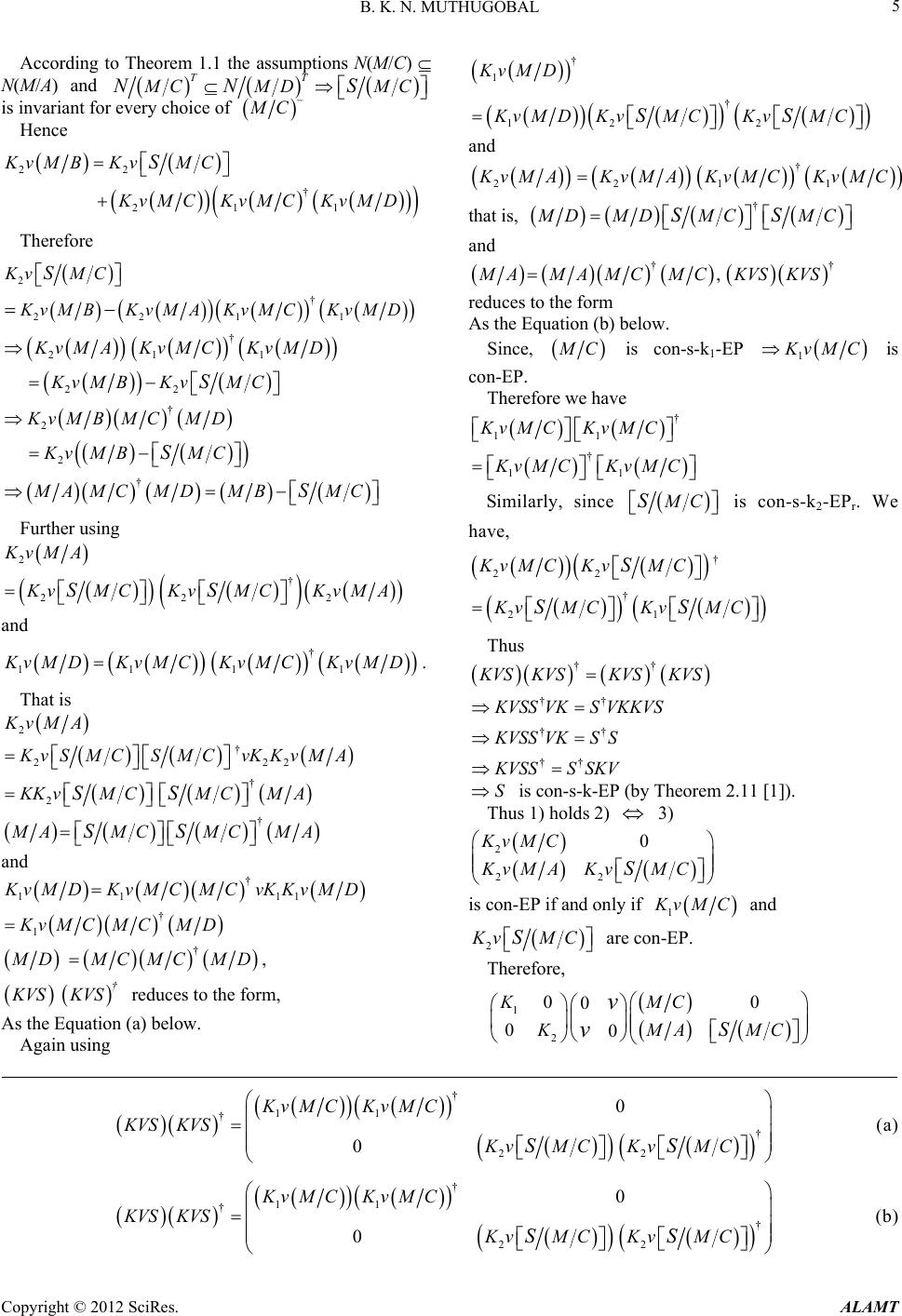 B. K. N. MUTHUGOBAL 5 According to Theorem 1.1 the assumptions N(M/C) N(M/A) and TT M CMD MNN SC is invariant for every choice of M C Hence 22 † 211 KνMB KνMC KνMC KνMC KνMD S Therefore 2 † 2211 KνMC KνMB KνMA KνMC Kν M D S † 21 1 22 KνMAKνMC Kν M D KνMB KνMC S † 2 2 KνMB MCMD KνMB MC S † M AMC MDMBMCS Further using 2 † 22 2 KνMA KνMCKν M CKvMASS and † 1111 KνMD KνMC Kν M CKvMD. That is 2 † 22 † 2 KνMA KνSMCSMC νKKν 2 M A KK νMCMCMA SS † M AMCMCMSS A and † 11 11 † 1 KνMD KνMC MC νKKν M D KνMC MCMD † M DMCMCMD, K VS † K VS reduces to the form, As the Equation (a) below. Again using † 1 † 12 2 KνMD KνMD KνMCKνMC SS and † 2211 KνMA KνMAKνMC Kν M C that is, † M DMDMCMCSS and †† , M AMAMCMCKVSKVS reduces to the form As the Equation (b) below. Since, M C is con-s-k1-EP 1 Kν M C is con-EP. Therefore we have † 11 † 11 KνMC KvMC K vMC KvMC Similarly, since M CS is con-s-k2-EPr. We have, † 22 † 21 KνMC KνMC KνMC KνMC S SS Thus †† K VS KVSKVSKVS †† †† †† K VSS VKS VKKVS KVSSVKSS KVSSS SKV S is con-s-k-EP (by Theorem 2.11 [1]). Thus 1) holds 2) 3) 2 22 0KνMC KνMA KνMC S is con-EP if and only if 1 Kν M C and 2 Kν M CS are con-EP. Therefore, 1 2 0 00 00 MC K MA MC KS ν ν † 11 † † 22 0 0 KνMCKνMC KVS KVS KνMC KνMC SS (a) † 11 † † 22 0 0 KνMCKνMC KVS KVS KνMC KνMC SS (b) Copyright © 2012 SciRes. ALAMT 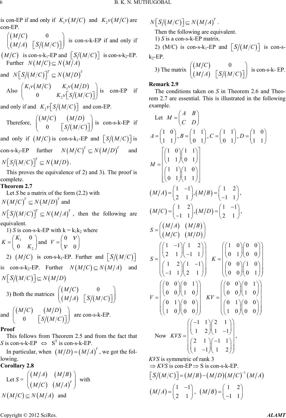 B. K. N. MUTHUGOBAL 6 is con-EP if and only if 1 Kν M C and 2 Kν M Care con-EP. 0MC MA MC S is con-s-k-EP if and only if M C is con-s-k1-EP and M CS is con-s-k2-EP . Further NMC NMA and TT NMCNMDS Also 11 2 0 KνMC KνMD KνSMC is con-EP if and only if and 2 KνSMC and con-EP. Therefore, 0 MC MD SMC is con-s-k-EP if and only if M Cis con-s-k1-EP and SMC is con-s-k2-EP further TT NMC NMD and T NS MCNMD . This proves the equivalence of 2) and 3). The proof is complete. Theorem 2.7 Let S be a matrix of the form (2.2) with TT NMC NMD and TT NMCNMAS , then the following are equivalent. 1) S is con-s-k-EP with k = k1k2 where 1 2 0 0 K K K and 0 0 Vν ν 2) M C is con-s-k1-EP. Further and M CS is con-s-k2-EP. Further NMC NMA and NMCNMDS 3) Both the matrices 0MC MA MC S and 0 MC MD SMC are con-s-k-EP. Proof This follows from Theorem 2.5 and from the fact that S is con-s-k-EP S T is con-s-k-EP. In particular, when T M DMA, we got the fol- lowing. Corollary 2.8 Let S = T M AMB MCM A with NMC NMA and T A. uiva NMCNMS Then the following are eqlent. 1) S is a con-s-k-EP matrix. d 2) (M/C) is con-s-k1-EP an M CS is con-s- k2 e matrix -EP. 3) Th 0MC MA MC S is con-s-k- EP. Rons taken on S in Theorem 2.6 and Theo- emark 2.9 The conditi rem 2.7 are essential. This is illustrated in the following example. Let A B MCD 1 0 11 A , 11 01 B ,11 01 C ,10 11 D 10 11 11 01 1110 0111 M 11 12 , 21 11 MA MB , 121 1 , 112 1 MCMD , M AMB S M CMD 1112 21 11 121 1 11 21 S 1000 01 00 0010 0001 K 0001 0010 01 00 1000 V 0001 0010 01 00 1000 KV Now KVS is symmetric of rank 3 s-k-EP. 11 21 121 1 21 11 1112 KVS , KVS is con-EPS is con- 1 M CM MDMCB MAS 11 21 MA , 12 11 MB Copyright © 2012 SciRes. ALAMT 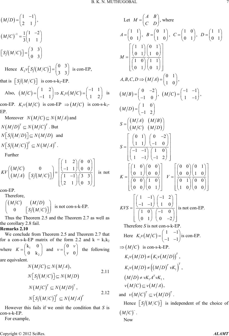 B. K. N. MUTHUGOBAL 7 11 21 MD , 112 1 11 3 MC 33 03 SMC Hence 2 03 33 KνSMC is con-EP, that is S MC is con-s-k2-EP. , Also 1 12 11 KνM 11 1 2 MCC is con-EP. 1 Kν M C is con-EP M C is con-s- EP. ver k1- Moreo C NMA NM and TT NMC . But NMD NS MDNMD and T NS MCNMA Further . T 1200 011 00 1133 21 03 KV MAS MC MC is not con-EP. Therefore, 0 MCMD SMC is not con-s-k-EP. Thus the Theorem 2.5 as well as the corollary 2.8 fail. Rrem 2.5 and Theorem 2.7 that P matrix of the form 2.2 and k = k1k2 ivalent. nd the Theorem 2.7 a emarks 2.10 We conclude from Theo for a con-s-k-E where 1 2 k0 0k K and 0 0 ν νν the following are equ ,NMC NMA NS MCNMD 2.11 , T TT NMC NMD NS MCNMA T 2.12 However this fails if we omit the condition t con-s-k-EP. hat S is For example, Let A B D MC , where , , 1 1 , 1 01 A 0 10 B 10 01 C 11 01 D 11 01 01 10 10 11 01 01 M 01 ,,, 10 ABCDM A , 02 10 MB , 11 11 MC , 10 12 MD M AMB S M CMD 010 2 111 0 11 10 11 12 S 10 00 01 00 00 10 00 01 K 00 01 00 10 01 00 10 00 V 11 12 11 10 1010 0102 KVS is not con-EP. Therefore S is not con-s-k-EP. Here 11 KνMC 111 P. is con-E M C is con-s-k-EP. 11 T KνMD KνMD, 11 T T KνMDMDνK, 11 T MD νKA ν K , νMC ν M A, and TT νMC ν M D. He SMC is iependent of the choice of ndnce M C . Now Copyright © 2012 SciRes. ALAMT 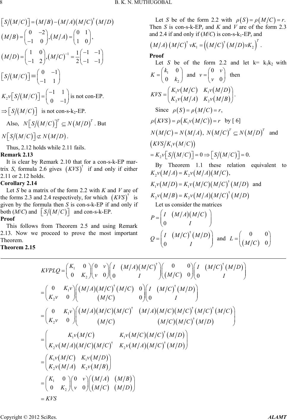 B. K. N. MUTHUGOBAL Copyright © 2012 SciRes. ALAMT 8 Let S be of the form 2.2 with .ρSρ M Cr Then S is con-s-k-EPr and K and V are of the form 2.3 and 2.4 if and only if (M/C) is con-s-k1-EPr and † SMCMBMAMC MD 02 01 , 10 10 MB MA , †† 12 T MAMC νKMCMDνK. 1 101 1 1 , 121 1 2 MD MC Proof Let S be of the form 2.2 and let k= k1k2 with and then 1 2 0 0 k Kk 0 0 ν νν 01 11 SMC 11 22 KνMC Kν M D KVS KνMAKν M B . 2 11 01 KνSMC is not con-EP. Since ,ρSρ M Cr SMC is not con-s- Also, k2-EP. 1 ρKVS ρKν M Cr by [ 6] TT NS MCNMD . But ,NMC NMA TT NMC NMD and NCNMD . Thus, 2.12 ho lds while 2.1 fails. Remark 2.13 r a con-s-k-EP mar- 2.6 gives S M 1 200 KVSKνMC KνSMC SMC 1. It is clear by Remark 2.10 that fo †By Theorem 1.1 these relation equivalent to 22 ,KνMA Kν M AMC trix S, formula K VS if and only if either 2. of the form 2.2 with K and V are of d 2.4 respectively, for wh ich 11 or 2.12 holds. Corollary 2.14 Let S be a matrix † 11 KνMD Kν M CMCMD and † 22 KνMBKν M AMC MD † K VS the forms 2.3 an is given by the formula then S is con-s-k-EP if and only if both (M/C) and SMC and con-s-k-EP Proof This follows em 2.5 and using . Let us consider the matrices 0 IMAMC P I from TheorRemark ow we proceed to prove the most important Th 2.13. N † 0 I MC MD Q I and 00 0 LMC eorem. Theorem 2.15 †† 1 2 †† 1 2 ††† 1 † 2 † 11 † 22 00 00 0 0000 00 000 0 0 Kν I MA MCIMCMD KVPLQ MC KνII KνMA MCMCIMCMD KνMC I MAMCMCMAMC MCMCMC Kν KνMCMC MCMD KνMC KνMC MCMD KνMA MCMCK † 11 22 1 2 00 00 νMA MCMD KνMC KνMD KνMA KνMB KMAMB ν KMCMD ν KVS  B. K. N. MUTHUGOBAL 9 Thus KVS can be factorized as KVS = KVPLQ. Since KVP = (KVQ)T. We have KVPTVK=Q. Therefore, T T T K VSKVPLKVP VK K VP LKVKVP K VP KVL KVP [since LVK = KVL]. Since (M/C) is con-s-k1-EPr. We have k1v(M/C) is con-EPr. Therefore (Theorem 2.11 of [1]) By Theorem 1.3 assume that S is con-s-k-EPr. Since S is con-s-k-EPr, KVS is con-EPr. Since KVS = KVPLQ, one choic e o f () T NLN LVK T NKVL NKVL TT NKVP KVLKVPNKVP KVLKVP T () T NKVSN KVS T NS NSVK S is con-s-k-EP (Theorem 2.11 of [1]). Since ρSr, S is con-s-k-EPr. Conversely, let us 11 † 00 0 K VSQPVK KVS MC is con-EP () T NKVSN KVS By Theorem 1.1 T . T K VS KVSKVSKVS That is, 11 22 νMAKν 11 22 T T MC KνMD KMB KνMC KνMD KνMAKνMB Kν 1† 00 0 QMC 1 2 11 KνMC Kν 2 M D PνMA VK KKν M B As the equation (at the bottom of this page). or conversely, † 11 TT KνMC Kν M CMCMC † 21 TT KνMC Kν M CMCMD and † 11 TT KνMC Kν M CMCMC From it follows that 1 T NMCN KνMC 1 T NMCNMC ν K MC is con-s-k-EP. Since .ρ M Cr M C is con-s-k-EPr. From † 21 TT KνMA Kν M CMCMD it follows that. Now, † 2 †† 1 †† 1 †† 1 † 1 † 1 T T T T TT T TT T KνMA MC MD MCKνMC MC MCMC MCKν MDMCMC MCνK MD MCνK KνMCMD (By theorem 2.11 [) T MD 1] †† 21 T KνMA MCMCMDν K †† 12 T MA MCνKKνMCMD † 12 T νKMCMDνK † MA MC Mark 2.16 hen (M/A) is non singlular, KV(M/A) is automti- cally con-EPr and (M/A) is con-s-k-EPr and Theorem 2.15 reo the following. Let S be of the form 2.2 with C non singular and Wa duces t Corollary 2.17 []ρSρ M C. Then S is con-s-k-EP with K = k1k2 and † 1 † 2 0 0 ν T νMAMCν K ν MC MDνK . † 11 1 † 22 11 TT TT TT TT KνMC KνMC Kν † MC MC 1 KνMA M † CMCMD KνMDKνMB KνMDMC MCKν M CMCMD Copyright © 2012 SciRes. ALAMT  B. K. N. MUTHUGOBAL 10 Remark 2.18 When k(i) = i, we have K1 = K2 = I, then the Theorem 2.15 reduces to the result for con-s-EP matrices. When KV = I then Theorem 2.15 reduces to Theorem 3 of [5]. Remark 2.19 Theorem 2.15 fails if we relax the condition on the rank of S. For example, let us consider the matrix S and K given in Remark 2.10, 2 But [][]ρKVSρS . 11,ρKVM CρMC 1 () ()ρKVS ρKνMA ρSρ. M A KVS is not con-EP Therefore S is not Con-s-k-EP. However, 1 100111 01 1011 011 111 10 1111 KVM C is con-EP. Therefore (M/C) is con-s-k1-EP and 111 1 11 2 MC , 1 1 11 1 11 2 A MCνK , M 110 MC MDνK . 210 = K1K2, where Thus the theorem fails. Corollary 2.20 Les S be a 2r x 2r matrix of rank r. Thus S is con-s-k-EPr with K 1 2 0 0 K K and V = 0 0 ν ν every secondary sub matrix of S of rank r is con-s-k-EPr. trix then KVS is an co ix by Theorem 2.11 [1]. Let Proof Suppose S is con-s-k-EPr ma n-EPr matr 1 Kν M C such thatbe any Principal submatrix of KVS 1 []ρKVS ρKν, M Cr tation matrix P such that, then there exists a permu- 11 22 TTKνMC Kν M D KVSPKVSPMA νKνK M B with 1.ρKVSρKν M Cr By [4] T K VS 2.15 that is con-EP . Now we conclude from Theorem r 1 Kν M C is con-EPr. That is (M/C) isr Si s under which a partitioned matrix is de k-EP matrices ale- mentary summands of S if S = S1 + S2 and con-s-k1-EP nce [M/C] is arbitrary it follows that every secondary submatrix of rank r is con-s-k-EPr. The converse is ob- vious. The condition composed into complementary sum and S of con-s- re given. S1 and S2 and called comp 12 .ρSρSρS Theorem 2.21 Let S be of the form 2.2 with ,ρSρMC ρSMC † (SMCMBMAMCMD where and K is of the form 2.3 and V is of the fo rm 2.4. If ( M/C) is con-s-k1-EP and SMC is con-s-k2-EP matrices such that †† 12 T MA MCνKMCMDνKand †† 21 T MDS MCνKSMCMCνK th Proof Let us consider the matrices, en S can be decomposed into complementary sum- mands of con-s-k-EP matrices. † †† 1 M CMCMCMD S M AMC MCMAMC MD and † 0IMCMC 2 †) MD SMA SM C IMCMC . toTaking in account that † M CNMAMCMA CvKNMA MCMCvKand †T NM 11 † 11 ††† 1 †† †† S MCMAMCMD MAM MAMC MDMAMCMCMC MD MA MCMDMAMCMC MAMC MMAMCMD †† CMDMC MCMCMD † MC MD 0 MC MC D Copyright © 2012 SciRes. ALAMT  B. K. N. MUTHUGOBAL 11 ain by [6] that We obt 1.ρSρ M C Since (M/C) is con-s-k1-EP and †† 1 † 1 † 1 †† T T C MC MCMC νK MA MCνK MC MDνK at is S is con-s-k1-EP. †† 1 M AMCMνK MA MC 2 MC MCMCMD νK We have by Theorem 2.15, th1 Since ,ρSρMC ρSMC Theorem 1 of [6], gives †,NS MCNIMCMCMD †T T NS MCNMCIMCMC and † † †0 IMCMC MDSMC IMC MC Therefore, 2 SSMC 0. Thus by [7] we get 2.ρSρSMC Thus 12 .ρSρSρS Further using † 11 MC MCKνKν M CMC We obtain, † † 2 †† †† 11 † † † † 11 †† 11 ( T TT TT TT T IMCMCMDSMCνK IMCMCSMC MAνKSMCvAνKIMC MC S MCvAIMCMCKνSMC vAKνMC MC Kν SMCMAKνKνMC MC 1 AIMCC νK †† 1 † 1 T T T T T SMCMAKνIMCMC M REFERENCES [1] S. Krishnamoorthy, K. Gunasekaran and B. K. N. Mut- hugobal, “con-s-k-EP Matries,” Journal of Mathematical Sciences and Engineering Applications, Vol. 5, No. 1, 2011, pp. 353-364. [2] C. R. Rao and S. K. Mitra, “Generalized Inverse of Ma- trices and Its Applications,” Wiley and Sons, New York, 1971. [3] ar ix Equations,” Mathematical Proceedings of the , Vol. 521, 1959, [4] T. S. Baskett and I. J. Katz, “Theorems on Products of EPr Matrices,” Linear Algebra and Its Applicationsol. 2, No. 1, 1969, pp. 87-103. A. R. Meenakshi, “On Schur Complements in an EP Ma- trix, Periodica, Mathematica Hungarica,” Periodica Mathematica Hungarica, Vol. 16, No. 3,, pp. 193- 200. [6] D. H. Carlson, E. Haynesworth and T. H. Markham, “A ation of the Schur Complme nt by Means of t he nrose Inverse,” SIAM Journal on Applied Ma- , 1974, pp. 169-175. [7] Greviue, “Generalized Invers Theory and Applications,” Wiley and Sons, New York, [8] y, K. Gunasekaran and B. K. N. Mut- hugobal, “On Sums of con-s-k-EP Matrix Thai Journal atics, in Press, 2012. † SM C M R. Penrose, “On Best Approximate Solutions of Line Matr , No. Cambridge Philosophical Society pp. 17-19. , V [5] 1985 Generaliz e Moore-Pe thematics, Vol. 26, No. 1 A. B. Isral and T. N. E.es 1974. S. Krishnamoorth,” of Mathem Copyright © 2012 SciRes. ALAMT |