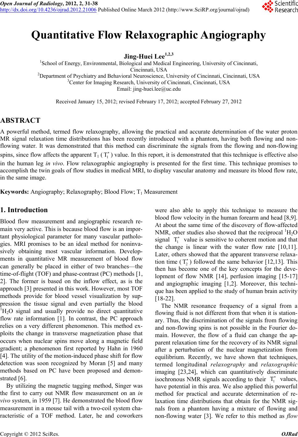
 Open Journal of Radiology, 2012, 2, 31-38 http://dx.doi.org/10.4236/ojrad.2012.21006 Published Online March 2012 (http://www.SciRP.org/journal/ojrad) Quantitative Flow Relaxographic Angiography Jing-Huei Lee1,2,3 1School of Energy, Environmental, Biological and Medical Engineering, University of Cincinnati, Cincinnati, USA 2Department of Psychiatry and Behavioral Neuroscience, University of Cincinnati, Cincinnati, USA 3Center for Imaging Research, University of Cincinnati, Cincinnati, USA Email: jing-huei.lee@uc.edu Received January 15, 2012; revised February 17, 2012; accepted February 27, 2012 ABSTRACT A powerful method, termed flow relaxography, allowing the practical and accurate determination of the water proton MR signal relaxation time distributions has been recently introduced with a phantom, having both flowing and non- flowing water. It was demonstrated that this method can discriminate the signals from the flowing and non-flowing spins, since flow affects the apparent T1 (T) value. In this report, it is demonstrated that this technique is effective also in the human leg in vivo. Flow relaxographic angiography is presented for the first time. This technique promises to accomplish the twin goals of flow studies in medical MRI, to display vascular anatomy and measure its blood flow rate, in the same image. 1 T Keywords: Angiography; Relaxography; Blood Flow; T1 Measurement 1. Introduction Blood flow measurement and angiographic research re- main very active. This is because blood flow is an impor- tant physiological parameter for many vascular patholo- gies. MRI promises to be an ideal method for noninva- sively obtaining most vascular information. Develop- ments in quantitative MR measurement of blood flow can generally be placed in either of two branches—the time-of-flight (TOF) and phase-contrast (PC) methods [1, 2]. The former is based on the inflow effect, as is the approach [3] presented in this work. However, most TOF methods provide for blood vessel visualization by sup- pression the tissue signal and even partially the blood 1H2O signal and usually provide no direct quantitative flow rate information [1]. In contrast, the PC approach relies on a very different phenomenon. This method ex- ploits the change in transverse magnetization phase that occurs when nuclear spins move along a magnetic field gradient; a phenomenon first reported by Hahn in 1960 [4]. The utility of the motion-induced phase shift for flow detection was soon recognized by Moran [5] and many methods based on PC have been proposed and demon- strated [6]. By utilizing the magnetic tagging method, Singer was the first to carry out NMR flow measurement on an in vivo system, in 1959 [7]. He demonstrated the blood flow measurement in a mouse tail with a two-coil system cha- racteristic of a TOF method. Later, he and coworkers were also able to apply this technique to measure the blood flow velocity in the human forearm and head [8,9]. At about the same time of the discovery of flow-affected NMR, other studies also showed that the reciprocal 1H2O signal 1 value is sensitive to coherent motion and that the change is linear with the water flow rate [10,11]. Later, others showed that the apparent transverse relaxa- tion time (2 T ) followed the same behavior [12,13]. This then has become one of the key concepts for the deve- lopment of flow NMR [14], perfusion imaging [15-17] and angiographic imaging [1,2]. Moreover, this techni- que has been applied to the study of human brain activity [18-22]. The NMR resonance frequency of a signal from a flowing fluid is not different from that when it is station- ary. Thus, the discrimination of the signals from flowing and non-flowing spins is not possible in the Fourier do- main. However, the flow of a fluid can change the ap- parent relaxation time for the recovery of its NMR signal after a perturbation of the nuclear magnetization from equilibrium. Recently, we have shown that techniques, termed longitudinal relaxography and relaxographic imaging [23,24], which can quantitatively discriminate isochronous NMR signals according to their 1 T values, have potential in this area. We also applied this powerful method for practical and accurate determination of re- laxation time distributions that obtain for the NMR sig- nals from a phantom having a mixture of flowing and non-flowing water [3]. We refer to this method as flow C opyright © 2012 SciRes. OJRad 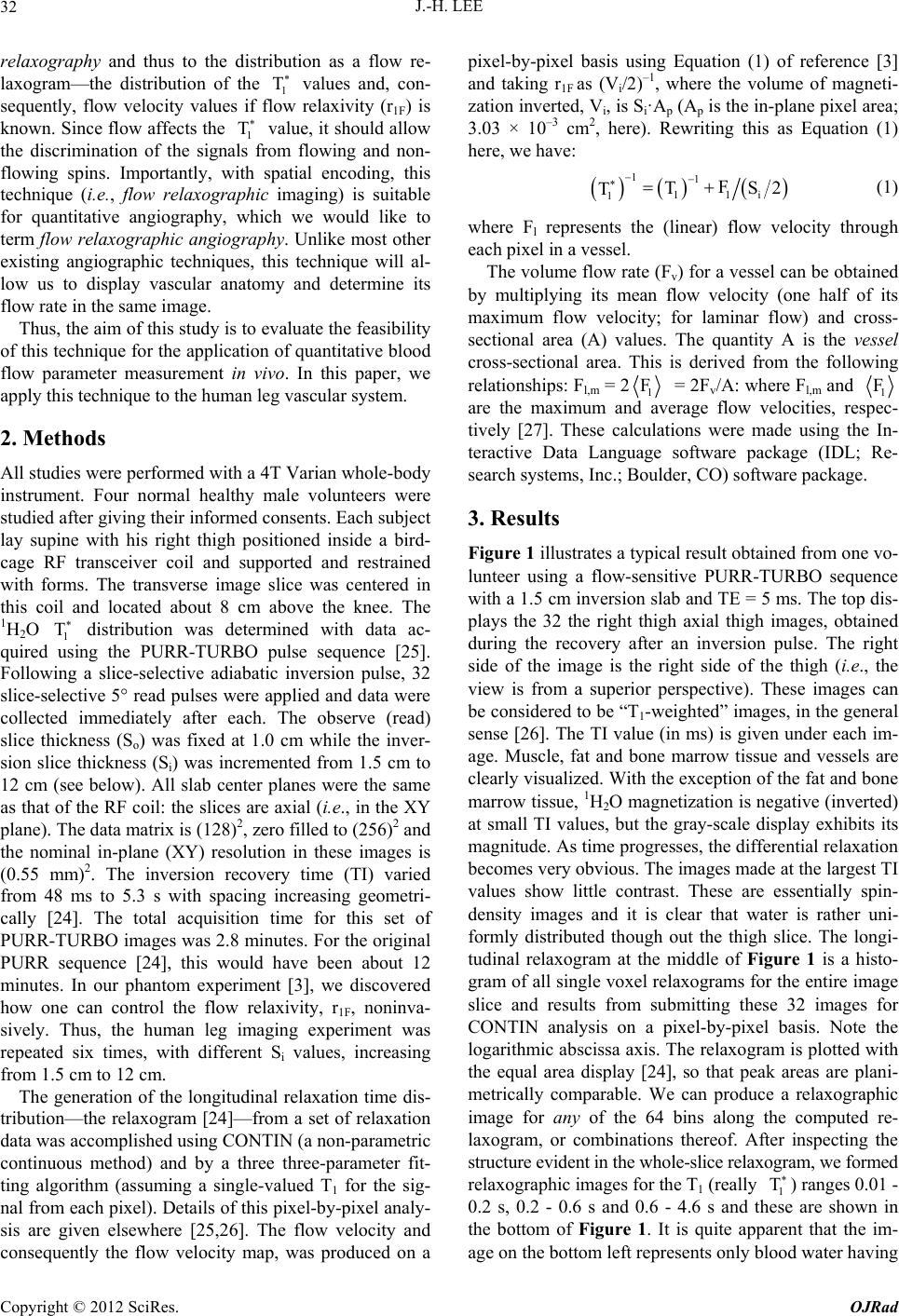 J.-H. LEE 32 relaxography and thus to the distribution as a flow re- laxogram—the distribution of the 1 values and, con- sequently, flow velocity values if flow relaxivity (r1F) is known. Since flow affects the 1 value, it should allow the discrimination of the signals from flowing and non- flowing spins. Importantly, with spatial encoding, this technique (i.e., flow relaxographic imaging) is suitable for quantitative angiography, which we would like to term f low relaxographic angiography. Unlike most other existing angiographic techniques, this technique will al- low us to display vascular anatomy and determine its flow rate in the same image. T T T Thus, the aim of this study is to evaluate the feasibility of this technique for the application of quantitative blood flow parameter measurement in vivo. In this paper, we apply this technique to the human leg vascular system. 2. Methods All studies were performed with a 4T Varian whole-body instrument. Four normal healthy male volunteers were studied after giving their informed consents. Each subject lay supine with his right thigh positioned inside a bird- cage RF transceiver coil and supported and restrained with forms. The transverse image slice was centered in this coil and located about 8 cm above the knee. The 1H2O 1 distribution was determined with data ac- quired using the PURR-TURBO pulse sequence [25]. Following a slice-selective adiabatic inversion pulse, 32 slice-selective 5° read pulses were applied and data were collected immediately after each. The observe (read) slice thickness (So) was fixed at 1.0 cm while the inver- sion slice thickness (Si) was incremented from 1.5 cm to 12 cm (see below). All slab center planes were the same as that of the RF coil: the slices are axial (i.e., in the XY plane). The data matrix is (128)2, zero filled to (256)2 and the nominal in-plane (XY) resolution in these images is (0.55 mm)2. The inversion recovery time (TI) varied from 48 ms to 5.3 s with spacing increasing geometri- cally [24]. The total acquisition time for this set of PURR-TURBO images was 2.8 minutes. For the original PURR sequence [24], this would have been about 12 minutes. In our phantom experiment [3], we discovered how one can control the flow relaxivity, r1F, noninva- sively. Thus, the human leg imaging experiment was repeated six times, with different Si values, increasing from 1.5 cm to 12 cm. The generation of the longitudinal relaxation time dis- tribution—the relaxogram [24]—from a set of relaxation data was accomplished using CONTIN (a non-parametric continuous method) and by a three three-parameter fit- ting algorithm (assuming a single-valued T1 for the sig- nal from each pixel). Details of this pixel-by-pixel analy- sis are given elsewhere [25,26]. The flow velocity and consequently the flow velocity map, was produced on a pixel-by-pixel basis using Equation (1) of reference [3] and taking r1F as (Vi/2)–1, where the volume of magneti- zation inverted, Vi, is Si·Ap (Ap is the in-plane pixel area; 3.03 × 10⁻³ cm2, here). Rewriting this as Equation (1) here, we have: 11 11i 1F TS2 T (1) where Fl represents the (linear) flow velocity through each pixel in a vessel. The volume flow rate (Fv) for a vessel can be obtained by multiplying its mean flow velocity (one half of its maximum flow velocity; for laminar flow) and cross- sectional area (A) values. The quantity A is the vessel cross-sectional area. This is derived from the following relationships: Fl,m = 21 = 2Fv/A: where Fl,m and F1 are the maximum and average flow velocities, respec- tively [27]. These calculations were made using the In- teractive Data Language software package (IDL; Re- search systems, Inc.; Boulder, CO) software package. F ) 3. Results Figure 1 illustrates a typical result obtained from one vo- lunteer using a flow-sensitive PURR-TURBO sequence with a 1.5 cm inversion slab and TE = 5 ms. The top dis- plays the 32 the right thigh axial thigh images, obtained during the recovery after an inversion pulse. The right side of the image is the right side of the thigh (i.e., the view is from a superior perspective). These images can be considered to be “T1-weighted” images, in the general sense [26]. The TI value (in ms) is given under each im- age. Muscle, fat and bone marrow tissue and vessels are clearly visualized. With the exception of the fat and bone marrow tissue, 1H2O magnetization is negative (inverted) at small TI values, but the gray-scale display exhibits its magnitude. As time progresses, the differential relaxation becomes very obvious. The images made at the largest TI values show little contrast. These are essentially spin- density images and it is clear that water is rather uni- formly distributed though out the thigh slice. The longi- tudinal relaxogram at the middle of Figure 1 is a histo- gram of all single voxel relaxograms for the entire image slice and results from submitting these 32 images for CONTIN analysis on a pixel-by-pixel basis. Note the logarithmic abscissa axis. The relaxogram is plotted with the equal area display [24], so that peak areas are plani- metrically comparable. We can produce a relaxographic image for any of the 64 bins along the computed re- laxogram, or combinations thereof. After inspecting the structure evident in the whole-slice relaxogram, we formed relaxographic images for the T1 (really 1 T ranges 0.01 - 0.2 s, 0.2 - 0.6 s and 0.6 - 4.6 s and these are shown in the bottom of Figure 1. It is quite apparent that the im- age on the bottom left represents only blood water having Copyright © 2012 SciRes. OJRad  J.-H. LEE Copyright © 2012 SciRes. OJRad 33 Figure 1. At the top are shown, 32 images obtained during the recovery of magnetization after an inversion RF pulse. The recovery time values (in ms) are indicated under each image. The nominal in-plane resolution is (0.55 mm)2. At the middle is a composite 1H2O longitudinal relaxogram (in logarithmic scale) representing data from every voxel in the entire image slice. Below it, also shown relaoxgraphic images made from the indicated sections (T1 values ranges) of the entire relaxogram. They illustrate naturally segmented images of tissues with different relaxation rate constants, as well as water with different flow rates. a large flow rate, mostly in the interior of larger vessel lumens (the popliteal artery (PA) and vein (PV), as well as two saphenous vessels (S1 and S2)); and the image on the bottom right represents only muscle tissue. However, the image in the bottom center is more complicated. It consists of bone marrow and subcutaneous fatty tissues, as well as blood water with a small flow rate. As we will see below, the rings in this image most likely represent the slow-flowing water near the vessel walls (i.e., vessel lumen annuli). Of course, the sum of all relaxographic images is the spin density image. It seems impressive that a very small vessel (arrow) buried in muscle can be also clearly visualized with relaxographic imaging, while not be seen easily (if at all) in the original T1-weighted  J.-H. LEE 34 images. Figure 2 center shows a stacked plot of the longitude- nal relaxogram from the same subject, as a function of Si. The relaxographic images (Si = 1.5 cm) of Figure 1 and their associated relaxogram are duplicated at the bottom of Figure 2 for comparison. Shown at the top of Fig- ure 2 are the Si = 12 cm relaxographic images, which are produced from the same T1 ranges as those of Figure 1. It is clearly seen that stationary 1H2O remains at the same T1 value regardless of the Si value. However, the T1 of flowing 1H2O is shifted to smaller values as Si decreases. The vessel with the greatest blood flow rate has the most reduced T1 value. Although the T1 value changes, it is important to note that the flow rate in each vessel does Figure 2. Shown at the middle is a stacked plot of the 1H2O longitudinal relaxogram as a function of inversion RF pulse slice thickness (Si). The majority of signal, which is from non-flowing muscle tissue water, remains unchanged as Si is altered; as illustrated with a vertical line. However, a very small amount of signal is shifted to smaller T1 values as Si decreases. As examples, the T1 changes for the popliteal artery (PA) lumen center and annulus are indicated. Relaxographic images (RIs) made from the same sections (indicated) of the bottom (Si = 1.5 cm) and the top (Si = 12 cm) relaxograms are shown below and above it, respectively. The RIs at the bottom are essentially duplicated from those in Figure 1. Comparison of the top and bottom images clearly shows that RIs with the same T1 value range are quite different. The RI at the top left represents essentially the noise in the case. Copyright © 2012 SciRes. OJRad  J.-H. LEE 35 not change. For Si = 12 cm, the relaxographic image, which has been windowed-up for clearness, from the smallest T1 range is essentially the noise for this case. The T1 value of the PA central lumenal 1H2O was deter- mined from the relaxogram at each Si value. These are indicated on the stacked plot. Also, a line is drawn con- necting the T1 values of the PA annular lumenal 1H2O at the largest Sis and that at 1.5 cm. The behavior observed helps confirm the assignment to water in the lumen an- nulus. Figure 3 depicts plots of 1 as functions of 2(Si)-1 for one pixel from each vessel seen in Figure 1 and the average 1 from 40 pixels selected at random from all muscle regions. The area of largest vessel, PV, contains almost 50 pixels, that of the smallest vessel detected, S3, contains almost 10 pixels. The 1 values are the recip- rocals of the 1 values for pixels selected from ROIs exhibiting the largest 1 values (i.e. the highest flow rate) of each vessel. Since the muscle 1 R values are quite uniform, we have chosen 40 pixels from muscle areas; a few pixels each from each muscle type and av- eraged their 1 values. The symbols represent data from five different vessels—PA, PV, subcutaneous saphenous veins (S1, S2, S3) —and muscle; from top to bottom, re- spectively. The solid lines drawn through them result from linear-least-squares (LLS) fittings. The root-mean- square, χ, values for all vessels are greater than 0.95 ex- cept for PA, for which it is 0.88. The slope value of each line essentially represents the maximum flow velocity (Fl,m) of each vessel. The volume flow rate (Fv, Ta ble 1) for each vessel can be obtained by multiplying its mean flow velocity ( R R R R R T 1 F = F1,m/2) and its cross-sectional area (A), which can be estimated from Figure 1 bottom center image. The vessel flow velocities measured in this study are quite reasonable and are in a very good agreement with those obtained by other investigators [28,29]. The flow rate of muscle water is of course essentially zero. The left panel of Figure 4 shows a color flow velocity map overlaid on a gray-scale anatomical image and the right panel shows a 3D plot of the PA and PV flow pat- terns. These were obtained by fitting the Si-dependent 1 data, on a pixel-by-pixel basis, with Equation (1). It is clear that the colored pixels represent only flowing water. We refer to the determination of the flow velocity map as flow relaxographic angiography. The map dis- plays vascular anatomy and vascular blood velocities simultaneously and quantitatively. In the 3-D flow pat- tern plot, the z-axis measures the linear flow velocity. The contour lines in the xy plane represent the 5, 10 and 15 cm/s flow rates. The flow patterns for these vessels are quite consistent with that of laminar flow. R Table 1 gives the measured cross-sectional area, the mean flow velocity and the volume flow rate for each vessel. It is interesting to note that for the vessels we can see the sum of the venous volume flow rates is almost equal to the arterial volume flow rate, which is physio- logically expected. Thus, the data in Tab le 1 can serve as a self-check for this technique. We also list for compari- son the calculated average intrinsic T1 (1) values from the ROIs indicated and their corresponding average measured T1 ( F 1 F ) values. The former are obtained from the average of the y-intercepts of the 1 R 2/Si- dependencies for all pixels within each of the vascular ROIs. The measured values were obtained for the same ROIs with the non-slice-selective inversion PURR- TURBO RF pulse sequence version. 4. Discussions We find it quite gratifying that this technique can differ- Figure 3. Plots of the 2/Si-dependence of the maximum first- order relaxation rate constant values obtained from single voxels in the selected regions indicated. The symbols repre- sent data from the popliteal artery and vein (PA, PV) and saphenous vessels (Ss), as well as the average of 1H2O 1 R values from muscles. The solid lines result from LLS fittings. Figure 4. A flow relaxographic angiography map and the corresponding flow pattern are shown. The left panel show s the color-coded map superimposed on the gray-scale anato- mic image of the same subject. On the right, the PA (the left peak) and PV (the right peak) 3D flow patterns are pre- sented. The three contour levels represent flow velocities of 5, 10, 15 cm/s, respectively. Copyright © 2012 SciRes. OJRad  J.-H. LEE 36 Table 1. Summary of the vascular and flow parameters and 1H2O T1 values. Vessel PA PV S1 S2 S3 Muscle Area (cm2) 0.14 0.16 0.045 0.038 0.031 N/A 1 F (cm/s) 9.0 5.3 4.6 3.5 0.8 0.04 +/– 0.01 Fv (mL/min) 76 51 12 8.0 1.5 N/A 1 T (s) 0.94 1.84 1.74 1.76 1.53 1.5 (NSS) (s) 0.68 1.61 1.55 1.45 1.18 1.4 1 T rentiate in space not only water signals from different tissues, but also from water with different flow velocities; that is, to observe the flow velocity distribution (flow patterns). We were also able to find the direct relation- ship (i.e., flow relaxivity) between water flow velocity and the relaxation rate constant. This allows us to convert relaxographic images into flow relaxographic angiogra- phic images, which display both vascular anatomy and its velocity simultaneously (Figure 4). The sum of all re- laxographic images is the spin-density image. The flow rates determined in this study (Table 1) are in good agreement with the analogous values obtained by Wehrli et al. [28] and Holland et al. [29]. The latter pa- per reported Doppler ultrasound measurements of the popliteal artery mean volume flow to be 72 mL/min (our observation, 76 mL/min). Wehrli et al. used a selective saturation-recovery spin-echo MRI method to measure the femoral vein mean flow velocity to be 5.25 cm/s (our measurement, 5.3 cm/s). Another important determination in this study is that of the T1 value of blood 1H2O, as if it was stationary in vivo, the average reciprocal value of the vertical axis intercept. As far as we are aware, this is the first time that the blood 1H2O T1 has been extrapolated to this condition. We have reported this in a flow phantom study [3]. It is conceivable that this value will not be the same as would be measured for stationary blood in vitro. It is important to note that the impossibly negative T1 vertical intercepts of Figure 3 result from the single voxel data plotted therein. When we analyze the average T1 value, 1, for the entire lumen of each vessel, we obtain positive intercepts [30]. This Figure 3 result can be attributed to insufficient magnetization inversion and/or greater flow rates at some regions near the lumens center. T The 1 extrapolations also yield the interesting observation that the value for the one artery studied (<1.0 s) is significantly less than those for 1H2O in the veins observed (averaging 1.72 sec) [30]. This is a rather a surprising result, since we (and probably most investiga- tors) would likely expect that their values should be very similar. Although, Radda and co-workers have shown that the state of blood oxygenation has a great impact on the in vitro transverse blood 1H2O relaxation rate con- stant at 1.5 T [31], it has a smaller effect on longitudinal relaxation at 4.7T [32]. This is because the change of the blood bulk magnetic susceptibility (BMS) caused by al- tering the deoxy-Fe concentration is significant, and while T2 is quite sensitive to this T1 is not. The water proton-iron electron dipolar (hyperfine) interaction is very small. Radda’s group also showed that the haema- tocrit value affects the 1H2O T2 values for oxygenated and deoxygenated blood in different ways. The former has a linear dependency caused by varying macromo- lecular concentration, while the latter has a much larger non-linear dependency because of the above mentioned BMS effect [31]. No evidence a haematocrit effect on T1 was shown. Even if it is true that T1 can be altered by the haematocrit, the difference we observe does not prove that the haematocrit is different between the blood in the artery and veins we examined. Thus, the T1 difference between the blood 1H2O in arteries and veins remains a very interesting question to be addressed. Further inves- tigations are clearly called for. Although Kauppinen and co-workers show that increasing the deoxygenation (as in veins) of in vitro blood does increase 1H2O R1 (i.e. de- crease T1), so does increasing the partial pressure of O2 for blood that is already well oxygenated (as in arteries) [32]. It is important to note that 1H2O T1 values in tissues are larger at higher field than at lower field [33]. Thus, with a 4T instrument, one will have a better chance to differentiate the NMR signals from flowing and non- flowing 1H2O, since the T1 of the former is always shifted to a smaller value, just as by a paramagnetic contrast reagent [34]. An important feature of the PURR family of pulse sequences is that the TI values are exponentially spaced [25], this provides us a highly dynamic range for T1 measurement during the period the magnetization be- comes fully recovered. It is impressive that a quite small vessel (arrowhead) embedded in the muscle group can be clearly visualized in the middle relaxographic image and not be easily seen (if at all) in the original T1-weighted images We can foresee a number of potential medical applications of this technique. For example, the study of vascular disease is obvious. It may also be possible to apply it to tumor diagnosis because the blood flow in tumor tissue is different than that in normal tissue. T In summary, we have demonstrated that the flow re- laxographic angiography is also effective in an in vivo system. And, as illustrated for the first time, it provides Copyright © 2012 SciRes. OJRad  J.-H. LEE 37 the possibility to display vascular anatomy and measure its blood flow rate on the same images—the twin goals of medical MRI flow studies—in the same image. 5. Acknowledgements We thank Dr. Charles S. Springer for helpful discussions and Dr. Manoj K. Sammi for assisting the initial work. REFERENCES [1] T. J. Masaryk, J. S. Lewin and G. Laub, “Magnetic Resonance Angiography,” In: D. D. Stark and W. G. Bradley, Eds., Magnetic Resonance Imaging, Mosby-Year Book, St. Louis, 1992, pp. 299-334. [2] E. M. Haacke, W. Lin and D. Li, “Flow in Whole Body Magnetic Resonance,” In: D. M. Grant and R. K. Harris, Eds., Encyclopedia of Nuclear Magnetic Resonance, John Wiley & Sons, New York, Vol. 3, 1996, pp. 2037-2047. [3] J.-H. Lee, X. Li, M. K. Sammi and C. S. Springer, “Using Flow Relaxography to Elucidate Flow Relaxivity,” Jour- nal of Magnetic Resonance, Vol. 136, No. 1, 1999, pp. 102-113. doi:10.1006/jmre.1998.1629 [4] E. L. Hahn, “Detection of Sea-Water by Nuclear Preces- sion,” Journal of Geophysical Research, Vol. 65, No. 2, 1960, pp. 776-777. doi:10.1029/JZ065i002p00776 [5] P. R. Moran, “A Flow Velocity Zeugatographic Interlace for NMR Imaging in Humans,” Magnetic Resonance Im- aging, Vol. 1, No. 4, 1982, pp. 197-203. doi:10.1016/0730-725X(82)90170-9 [6] J. W. Van Goethem, L. van den Hauwe, O. Ozsarlak and P. M. Parizel, “Phase-Contrast Magnetic Resonance An- giography,” JBR-BTR, Vol. 86, 2003, pp. 340-344. [7] J. R. Singer, “Blood Flow Rates by Nuclear Magnetic Resonance Measurements,” Science, Vol. 130, 3389, 1959, pp. 1652-1653. doi:10.1126/science.130.3389.1652 [8] O. C. Morse and J. R. Singer, “Blood Velocity Measure- ments in Intact Subjects,” Science, Vol. 170, No. 3956, 1970, pp. 440-441. doi:10.1126/science.170.3956.440 [9] J. R. Singer and L. E. Crooks, “Nuclear Magnetic Reso- nance Blood Flow Measurements in the Human Brain,” Science, Vol. 221, No. 4611, 1983, pp. 654-656. doi:10.1126/science.6867733 [10] P. M. Denis, G. J. Béné and R. C. Exterman, “Steady- State Observation of a Transitory Nuclear Resonance Phenomenon,” Archives of Sciences, Vol. 5, 1952, pp. 32- 34. [11] J. R. Singer, “Flow Rates Using Nuclear or Electron Paramagnetic Resonance Techniques with Applications to Biological and Chemical Processes,” Journal of Applied Physics, Vol. 31, No. 1, 1960, pp. 125-127. doi:10.1063/1.1735386 [12] M. A. Hemminga, P. A. De Jager and A. Sonneveld, “The Study of Flow by Pulsed Nuclear Magnetic Resonance. I. Measurement of Flow Rates in the Presence of a Station- ary Phase Using a Difference Method,” Journal of Mag- netic Resonance, Vol. 27, 1977, pp. 359-370. [13] J. R. Singer, “NMR Diffusion and Flow Measurements and an Introduction to Spin Phase Graphing,” Journal of Physics E: Scientific Instruments, Vol. 11, No. 4, 1978, pp. 281-291. doi:10.1088/0022-3735/11/4/001 [14] H. C. Dorn, “Flow NMR,” In: D. M. Grant and R. K. Harris, Eds., Encyclopedia of Nuclear Magnetic Reso- nance, John Wiley & Sons, New York, Vol. 3, 1996, pp. 2026-2036. [15] R. R. Edelman, H. P. Mattle, J. Kleefield and M. S. Silver, “Quantification of Blood Flow with Dynamic MR Imag- ing and Presaturation Bolus Tracking,” Radiology, Vol. 171, 1989, pp. 551-556. [16] J. A. Detre, J. S. Leigh, D. S. Williams and A. P. Koret- sky, “Perfusion Imaging,” Magnetic Resonance in Medi- cine, Vol. 23, No. 1, 1992, pp. 37-45. doi:10.1002/mrm.1910230106 [17] K. K. Kwong, D. A. Chesler, R. M. Weisskoff, K. M. Donahue, T. L. Davis, L. Ostergaard, T. A. Campbell and B. R. Rosen, “MR Perfusion Studies with T1 Weighted Echo Planar Imaging,” Magnetic Resonance in Medicine, Vol. 34, No. 6, 1995, pp. 878-887. doi:10.1002/mrm.1910340613 [18] R. R. Edelman, B. Siewert, D. G. Darby, V. Thangaraj, A. C. Nobre, M. M. Mesulam and S. Warach, “Qualitative Mapping of Cerebral Blood Flow and Functional Local- ization with Echo Planar MR Imaging and Signal Target- ing with Alternating Radio Frequency,” Radiology, Vol. 192, No. 2, 1994, pp. 513-520. [19] K. K. Kwong, “Functional Magnetic Resonance Imaging with Echo Planar Imaging,” Magnetic Resonance Quar- terly, Vol. 11, No. 1, 1995, pp. 1-20. [20] S.-G. Kim, “Quantification of Relative Blood Flow Change by Flow-Sensitive Alternating Inversion Recov- ery (Fair) Technique: Application to Functional Map- ping,” Magnetic Resonance in Medicine, Vol. 34, No. 3, 1995, pp. 293-301. doi:10.1002/mrm.1910340303 [21] S.-G. Kim and N. V. Tsekos, “Perfusion Imaging by a Flow-Sensitive Alternating Inversion Recovery (Fair) Technique: Application to Functional Brain Imaging,” Magnetic Resonance in Medicine, Vol. 37, No. 3, 1997, pp. 425-435. doi:10.1002/mrm.1910370321 [22] E. C. Wong, R. B. Buxton and L. R. Frank, “Implementa- tion of Quantitative Perfusion Imaging Techniques for Functional Brain Mapping Using Pulsed Arterial Spin Labeling,” NMR in Biomedicine, Vol. 10, No. 4-5, 1997, pp. 237-249. doi:10.1002/(SICI)1099-1492(199706/08)10:4/5<237::AI D-NBM475>3.0.CO;2-X [23] J.-H. Lee, C. Labadie, C. S. Springer and G. S. Harbinson, “Two-Dimensional Inverse Laplace Transform NMR: Altered Relaxation Times Allow Detection of Exchange Correlation,” Journal of the American Chemical Society, Vol. 115, No. 17, 1993, pp. 7761-7764. doi:10.1021/ja00070a022 [24] C. Labadie, J.-H. Lee, G. Vétek and C. S. Springer, “Re- laxographic Imaging,” Journal of Magnetic Resonance, Series B, Vol. 105, No. 2, 1994, pp. 99-112. doi:10.1006/jmrb.1994.1109 [25] J.-H. Lee, “PURR-TURBO: A Novel Pulse Sequence for Longitudinal Relaxographic Imaging,” Magnetic Reso- Copyright © 2012 SciRes. OJRad  J.-H. LEE Copyright © 2012 SciRes. OJRad 38 nance in Med icine, Vol. 43, No. 5, 2000, pp. 773-777. doi:10.1002/(SICI)1522-2594(200005)43:5<773::AID-M RM23>3.0.CO;2-7 [26] M. K. Sammi, C. A. Felder, J. S. Fowler, J.-H. Lee, A. V. Levy, X. Li, J. Logan, I. Palyka, W. D. Rooney, N. D. Volkow, G.-J. Wang and C. S. Springer, “The Intimate Combination of Low- and High-Resolution Image Data: I. Real-Space PET and 1H2O MRI, PETAMRI,” Magnetic Resonance in Medicine, Vol. 42, No. 2, 1999, pp. 345- 360. doi:10.1002/(SICI)1522-2594(199908)42:2<345::AID-M RM17>3.0.CO;2-E [27] M A. Hemminga, “Measurement of Flow Characteristics Using Nuclear Magnetic Resonance,” In: T. L. James and A. R. Margulis, Eds., Biomedical Magnetic Resonance, Radiology Research and Education Foundation, San Francisco, 1984, pp. 157-184. [28] F. W. Wehrli, A. Shimakawa, J. R. MacFall, L. Axel and W. Perman, “MR Imaging of Venous and Arterial Flow by a Selective Saturation-Resovery Spin Echo (SSRSE) Method,” Journal of Computer Tomography, Vol. 9, No. 3, 1985, pp. 537-545. doi:10.1097/00004728-198505000-00024 [29] C. K. Holland, J. M. Brown, L. M. Scoutt and K. J. W. Taylor, “Lower Extremity Volumetric Arterial Blood Flow in Normal Subjects,” Ultrasound in Medicine and Biology, Vol. 24, No. 8, 1998, pp. 1079-1086. doi:10.1016/S0301-5629(98)00103-3 [30] J.-H. Lee, M. K. Sammi and C. S. Springer, “Flow Re- laxographic Angiography,” Proceedings of the Interna- tional Society for Magnetic Resonance in Medicine, Vol. 8, 2000, p. 1828. [31] K. R. Thulborn, J. C. Waterton, P. M. Matthews and G. K. Radda, “Oxygenation Dependence of the Transverse Re- laxation Time of Water Protons in Whole Blood at High Field,” Biochimica et Biophysica Acta (BBA)—General Subjects, Vol. 714, No. 2, 1982, pp. 265-270. doi:10.1016/0304-4165(82)90333-6 [32] M. J. Silvennoinen, M. I. Kettunen and R. A. Kauppinen, “Effects of Hematocrit and Oxygen Saturation Level on Blood Spin-Lattice Relaxation,” Magnetic Resonance in Medicine, Vol. 49, No. 3, 2003, pp. 568-571. doi:10.1002/mrm.10370 [33] W. D. Rooney, G. Johnson, X. Li, E. R. Cohen, S. G. Kim, K. Ugurbil and C. S. Springer, “Magnetic Field and Tissue Dependencies of Human Brain Longitudinal 1H2O Relaxation in Vivo,” Magnetic Resonance in Medicine, Vol. 57, No. 2, 2007, pp. 308-318. doi:10.1002/mrm.21122 [34] T. E. Yankeelov, W. D. Rooney, W. Huang, J. P. Dyke, X. Li, A. Tudorica, J.-H. Lee, J. A. Koutcher and C. S. Springer, “Evidence for Shutter-Speed Variation in CR Bolus-Tracking Studies of Human Pathology,” NMR Biomedicine, Vol. 18. No. 3, 2005, pp. 173-185. doi:10.1002/nbm.938
|