International Journal of Modern Nonlinear Theory and Application, 2012, 1, 6-13
http://dx.doi.org/10.4236/ijmnta.2012.11002 Published Online March 2012 (http://www.SciRP.org/journal/ijmnta)
Chaotic and Hyperchaotic Complex Jerk Equations
Gamal M. Mahmoud, Mansour E. Ahmed
Department of Mathematics, Faculty of Science, Assiut University, Assiut, Egypt
Received January 27, 2012; revised February 29, 2012; accepted March 12, 2012
ABSTRACT
The aim of this paper is to introduce and investigate chaotic and hyperchaotic complex jerk equations. The jerk equa-
tions describe various phenomena in engineering and physics, for example, electrical circuits, laser physics, mechanical
oscillators, damped harmonic oscillators, and biological systems. Properties of these systems are studied and their Lya-
punov exponents are calculated. The dynamics of these systems is rich in wide range of systems parameters. The con-
trol of chaotic attractors of the complex jerk equation is investigated. The Lyapunov exponents are calculated to show
that the chaotic behavior is converted to regular behavior.
Keywords: Hyperchaotic; Chaotic; Attractors; Lyapunov Exponents; Jerk Function; Control; Complex
1. Introduction
Chaos and hyperchaos can occur in systems of autono-
mous ordinary differential equations (ODE’s) with at least
three variables and two quadratic nonlinearities [1-4]. The
Poincaré-Bendixson theorem shows that chaos does not
exist in a two-dimensional autonomous system. In 1994,
Sprott [5] found numerically fourteen chaotic systems
with six terms and one quadratic nonlinearities. In 1996,
Gottlieb [6] showed that some of these systems could be
written as a single third-order ODE. By “jerk function” he
means a function j such that the third-order ODE can be
written in the form

,,j


 
 , where j is the time
derivative of the acceleration

 and the equation is
called a jerk equation. The jerk equations describe various
phenomena in engineering and physics, for example,
electrical circuits, laser physics, mechanical oscillators,
damped harmonic oscillators, and biological systems. In
the literature some jerk equations are introduced and stu-
died [7-13]. Kocić et al. [14] considered and studied two
modifications of a 3-dimensional dynamic flow known as
jerk dynamical systems of Sprott [13].
In this paper, we define a complex jerk equation as an
autonomous third-order complex differential equation of
the form:

,,,,, ,zj zzzzzz
 

(1)
where z is a complex variable, the overdot represent the
time derivative and j is the complex jerk function (time
derivative of acceleration ) and an overbar denotes
complex conjugate variables. In recent years we intro-
duced and studied several complex nonlinear systems
which appear in many important applications [15-21].
z

As an example of Equation (1), we propose a chaotic
complex jerk equation as:
20zzzzzz


 
  (2)
where α, β and η, are positive parameters, ν is a negative
parameter, z is complex variable, dots represent deriva-
tives with respect to time and an overbar denotes com-
plex conjugate variables.
We suggest the equation:
20, 0,zzzzz


 
  (3)
which is an example of a hyperchaotic complex jerk equ-
ation. The corresponding real form of (3) (i.e. z is a real
variable) was introduced in [9], and has only chaotic be-
havior.
The organization of rest of the paper is as follows: In
Section 2, symmetry, invariance, fixed points of (2) and
stability analysis of the trivial fixed point are discussed.
Lyapunov exponents are calculated in Section 3, and
used to classify the attractors of (2). It is clear that our
Equation (2) has chaotic, periodic, quasi-periodic attract-
tors and solutions that approach fixed points. In Section 4,
we study the basic properties of the hyperchaotic com-
plex jerk Equation (3). Numerically the range of pa- ra-
meters values of the system at which hyperchaotic at-
tractors exist is calculated in Section 5. Section 6 con-
tains the control of chaotic attractors of Equation (2) by
adding a complex periodic forcing. The last section con-
tains our concluding remarks.
2. Basic Properties of Chaotic Jerk Equation (2)
In this section we study the basic properties of our new
Equation (2). Equation (2) can equivalently be written as
three, first-order, ordinary differential equations as:
C
opyright © 2012 SciRes. IJMNTA

G. M. MAHMOUD ET AL. 7
2
,,zxxyyyx z zz  
 ,
4
(4)
where
12
,zu iu 3
x
uiu and are
5
yu iu
6
complex variables, 1i, are real
variables, dots represent derivatives with respect to time
and an overbar denotes complex conjugate variables.
,1,2,,
j
uj6


The real version of (4) is:


13243546
22
5531112
22
6642212
,,,,
,
.
uuuuuuuu
uuuuuuu
uuuuuuu



 
  
 


(5)
The basic dynamical properties of system (5) are:
2.1. Symmetry and Invariance
From (5), we note that this system is invariant under the
transformation

123456123456
,,,,,,, ,, ,.uu uu uuuuuuuu 

,,,,,uuuuuu
Therefore, if is a solution of (5),
then 12 is also a solution of
the same system.
123456

3456
,,,uu uu,,uu
2.2. Dissipation
The divergence of (5) is:
6
1
2.
j
jj
u
u





Therefore the system (5) is dissipative for the case:
0.


2.3. Equilibria and Their Stability
The fixed points of system (5) can be found by solving
the following equations:


3456
22
5 31112
22
642212
0, 0, 0,0,
0,
0.
uu u u
uuuuuu
uuuuuu



 
 
(6)
Therefor system (4) has trivial fixed point

00,E
. The projection in the plane of the
non trivial fixed points is a circle:

0,0,0,0,0

12
,uu

22 2
12 ,uu r (7)
whose center is at the origin and radius is r

 .
The non trivial fixed point can be written in the form

123456
=,,,,,E uuuuuu

where 1cos ,ur


2sin ,ur


for
3456
0,uuu u


0, 2π  .
To study the stability of the Jacobian matrix of
Equation (2) at is:
0
E
0
E
0
0010 0 0
000 10 0
0000 1 0
.
0000 0 1
00
00 0
E
J

0









 


 

The characteristic polynomial is:

2
32 0.



  (8)
According to the Routh-Hurwitz condition, the real
parts of the roots

of (8) are negative if and only if
0,0, 0,0.

  
Since, 0


then is unstable.
0
The stability analysis of
E
E

can be similarly studied
as we did for the trivial fixed point .
0
E
3. Lyapunov Exponents and Attractors of
Equation (2)
This section is devoted to calculate Lyapunov exponents
and used their signs to classify attractors of Equation (2).
Based on these exponents, we compute parameters val-
ues of our Equation (2) at which chaotic, periodic, and
quasi-periodic attractors and attractors that approach
fixed point exist.
3.1. Lyapunov Exponents
System (5) in vector notation can be written as:




;,Ut hUt


 (9)
where
   
123456
,,,,, t Ut utututututut





123456
,,,,, ,
t
h hhhhhh is the state space vector,

is
a set of parameters and denoting transpose. The
equations for small deviations

t
U

from the trajectory


Ut are:






,U; 1,2,3,4,5,6
lj
UtLUt 
,lj
 
(10)
, where ,=l
lj
j
h
Lu

is the Jacobian matrix of the form:



,
22
12 12
22
122 1
00100
00 0100
00 0010
.
00000
32 0
2300
lj
L
uu uu
uuu u
 
0
1
0











 







G. M. MAHMOUD ET AL.
8
The Lyapunov exponents l

of the system is defined
by:


1
lim log.
0
l
ltl
ut
tu



 (11)
To find l

, Equations (9) and (10) must be numerically
solvedltaneously. Runge–Kutta method of order 4 simu
is used to calculate l

.
1, For thoicee ch 4, 5

   and 1

 and the
initial conditions






01
0, 04, tu

1 and
2 3
0 2,u 1, 0u 
 
45
02, 0uu


601u
ents which are: 0. 2
. Weate the
3
44, 0,
calcul
12
0, Lyapunov expon


.

45
0.488, 6 0.954, 1.691

  
at our system (4) for

This means th this cf α, β, hoice o
μ and η is a chaotic system since one of its Lyapunov
exponents 1

is positive and dissipative system because
their sum is negative.
3.2. Attractors of Equation (2)
3.2.1. Fix ,4

 ,5

 1


and Vary

In Figures 1(a) and (b) we plotted the corresponding
Lyapunov exponents λl, of system (5) us-
ing the initial conditions
1, 2,,6l
00,t

1 u

04 ,


201,u


01

302u ,

402u,

501u and 6
u

. It
is clear that from Figure 1(a), when


0.65,0.795 , 


0.840,1.025 and


1. 2 6
ors. It has
, 1. 3 4 the ne
also peri
w sy
odic a
stem (5) has
ttractors for chaotic attract


1. 3 4,2. 5  
when
4, while it has quasi-periodic attractors

lies in the interval


0.795,
oach nontri
. As is shown i
0.840
vial fixe
n
. Solutions
d points are
Figure 1(b) the
of system (5)
exist for
 
values of 4
that appr

2.54, 4.7
,

5

and 6

are negative.
3.2.2. Fix ,1

 ,5

 1


and Vary

has cFrom Figure that (5)haotic
attractors for
1(c) one can conclude


3.4, 3.590  ,


3.610,3.925,

3.955,

4.135 and


4.155, 4.880, and periodic attractors for β
lies in


3.590,3.610,


4.135, 4.155 and


4.
proach non

4.
880, 9.8.
trivial fixed Solutio
points are
ns of
exist
system (5) that ap
for 10.1,12  .
3.2.3. Fix ,1

 ,4

 1


and Vary

As we did bef1λ2 and λ3 in Figure 1(d)
and we see that (5) has chaotic attractors for
ore we plot only λ,


6.7, 6.315   ,


6.240,5.955,


5.865, 5.580 ,


5.525, 5.105,


5.07, 4.805 and


4.775,3.995 . In between above values of

our sys-
tractors as one sees from .
3.2.4. Fix
tem has periodic atFigure 1(d)
,1

 ,4

 5


 and Vary

rAs is showaotic attractos exist
for
n in Figure 1(e), the ch


0.001,1.14  
Using the same ch
.
oice of the parameters and initial
conditions as in Figure 1, the chaotic attractors of (5) are
plotted in Figure 2 in


234
,,uuu ,

246
,,uuu ,

2,u

45
,uu and


145
,,uu u spaces respectively.
4. Some Properties of Equation (3)
This section deals with the basic dynamical properties of
a hyperchaotic jerk Equation (3). As we did in Section 2,
Equation (3) can be written as a system of three, first-
order, ordinary differential equations such as:
,
2
,,zxxyyyzx z 


  (12)
where 12 3
, zu iuxuiu
4


riables,
and are com-
plex va
56
yu iu
1, ,1,2,
j
iuj 
on of (3) is:
, 6 are real variables.
The real versi
1
2


13243546
22
55134234
22
66234134
,,,,
2,
2.
uuuuuuuu
uuuuuuuuu
uuuuuuuuu



 

 
 


(13)
If


123456
,,,,,uuuuuu is a solution of (13), then

1,u


23456
,,,,uuuuu
From (13) if 0,
is also a solution.

 then (13) is dissipative.
System (13) has only trivial fixed point

00, 0,E
cobian

0,0,0,0
To stud
.
y the stability of we calculate the Ja
matrix of system (13) at get:
0
E
0 toE
0
00100 0
000100
00001 0
.
00000 1
1000 0
01000
E
J














Its characteristic polynomial is:
.


2
32
10P 


(14)
An elementary study proves that this polynomial has
only one real root 2
3
r



 which is therefore nega-
tive. Since the characteristic equation is a cubic equation
with real coefficients, we will have without loss of gen-
erality







rc
Pc

 . where c

is a
complex number. After expanding the above equation
and comparing the coefficients with those of the original
characteristic equation we come up with the relation


12
Re 2
cr




. We conclude that the real part of c

is
e fixed point is unstable, see Ref. [9
5. Lyapunov Exponents and Attractors of
Hyperchaotic Equation (3)
In this section we calculate the Lyapunov exponents and
attractors of Equation (3).
positive and that th].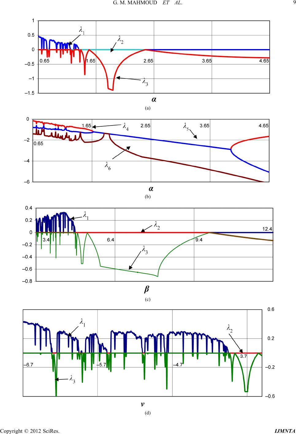

G. M. MAHMOUD ET AL. 9
(a)
(b)
(c)
(d)

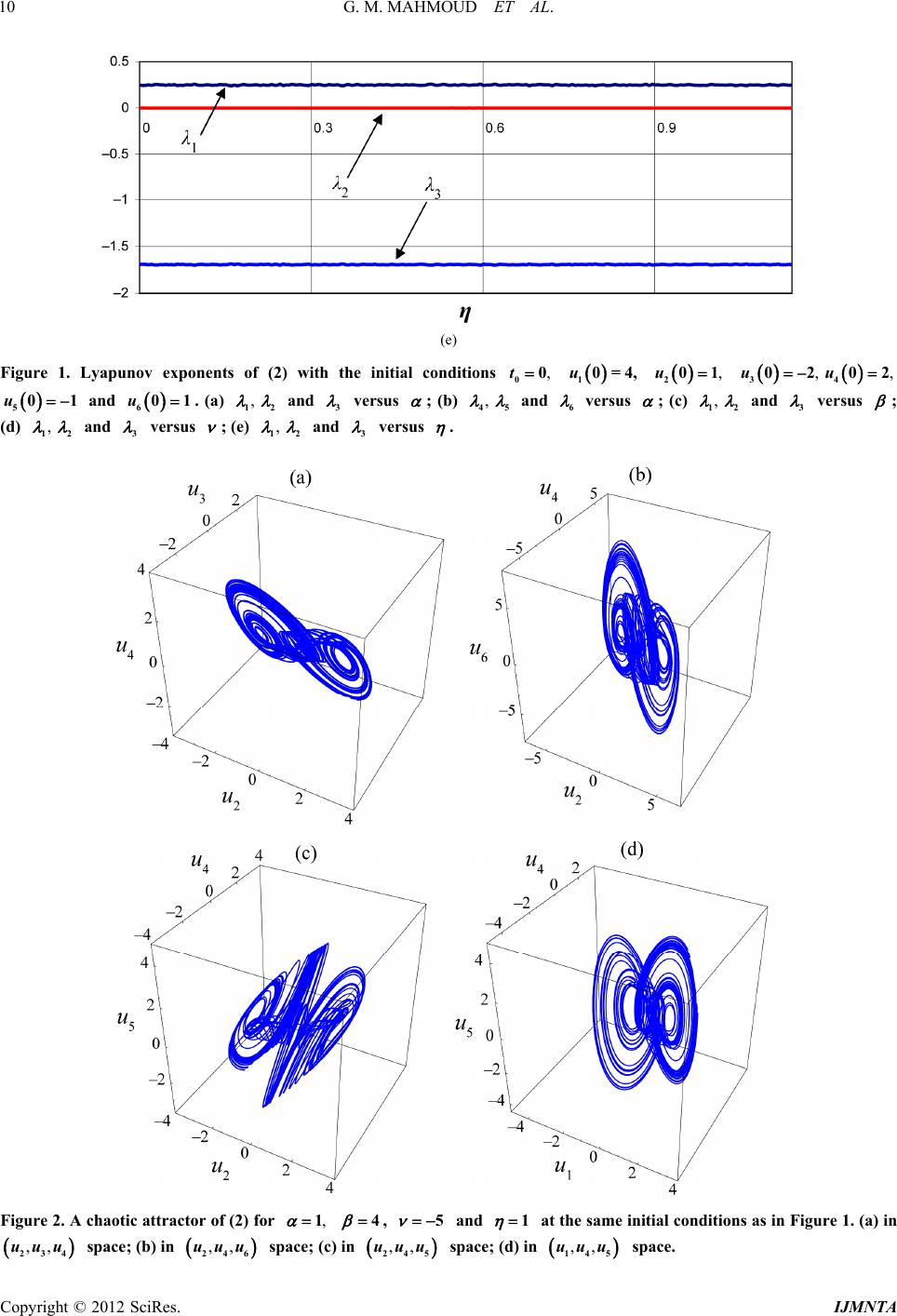G. M. MAHMOUD ET AL.
10
(e)




,
201u



, ,
34
0202uu
10=4,u , 00t

Figure 1. Lyapunov exponents of (2) with the initial conditions

501u d

601u. (a) , 12
an

 and 3

versus

; (b) ,
45

 and 6

versus

; (c) ,
12

 and 3

versus

;
(d) ,
12

 and 3

versus

; (e) ,
12

 and 3

versus

.
Figurttractor of (2) for ,1e 2. A chaotic a

 4


, 5


 and 1


at the same initial conditions as in Figure 1. (a) in

,,
234
uu space; (b) in

,,
246
uuu space; (c) in


,,
245
uuu uspace; (d) in


,,
145
uuu space.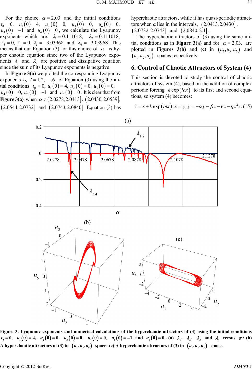

G. M. MAHMOUD ET AL.
11
For the choice 2.03


,

200u
and the initial conditions
,
00,t

104u,

300u


400u,

punov

5
u
exponents
01 and u
which

600
are: 1
, we cal
0.11
culate the Lya
1018,

 20.111018,


34
0, 
5
3.039680,

 and 63.03968


his choice of
. This
means that our Equation (3) for t

is hy-
nov expo- per cha
nents
otic equati
1
on since two of the Lyapu

and 2

e sum of
are positiv
its Lyapunov
e
ex
and dissipativ
ponents is ne
e equation
gative. since th
In Figure 3(a) we plotted the corresponding Lyapunov
exponents λl, of Equation (3) using the ini-
tial condition
1, 2,, 6l
s



2 3
4, 00, 00,u u
01
0, 0tu

01 and


45
00,uu


600u. It is clear that from
Figure 3(a), when




2.0278,2.0413 2.0430,2.0539

，,
Equation (3) has
hyperchaotic attractors, while it has quasi-periodic attract-
tors when α lies in the intervals,


2.0413, 2.0430,


2.0732, 2.0743 and


2.0840,
tractors o
2.1 .
f (3) using the samThe hyperchaotic ate ini-
tial conditions as in Figure 3(a) and for 2.03,


are
plotted in Figures 3(b) and (c) in and

235
,,uuu


123
,,uu u spaces respectively.
6. Control of Chaotic Attractors of System (4)
This section is devoted to study the control of chaotic
attractors of system (4), based on the addition ofomplex
periodic forcing
c


expkit

es:
to its first and second equa-
tions, so system (4) becom


2
exp, ,.zxkitxyyyxzzz   




2.0544, 2.0732 and


2.0743, 2.0840
 (15)
Figure 3. Lyapunov exponents and numerical calculations of the hyperchaotic attractors of (3) using the initial conditions
,t
00
 u
104,
 ,u
200
 ,u
300
 ,u

400

 u


501 and

 u

600. (a)

1,

2,

3 and

4 versus

; (b)
A hyperchaotic attractors of (3) in


uu
23
,,u
5
space; (c) A hyperchaotic of (3)attractors in


uuu
12
,,
3
space.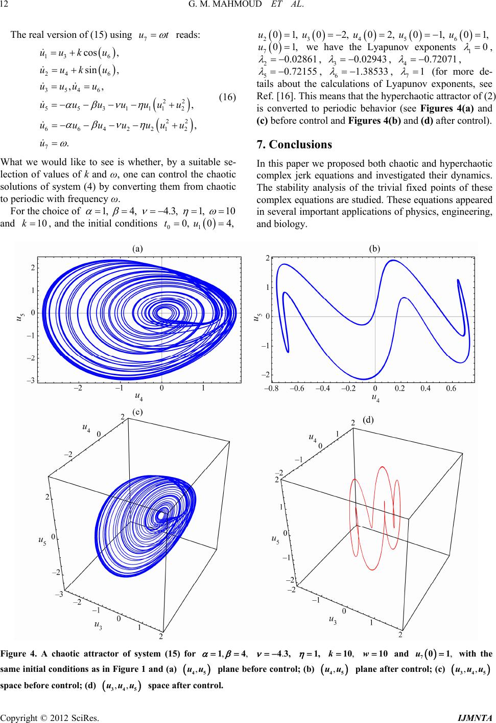

G. M. MAHMOUD ET AL.
12
The real version of (15) using 7 ut

 reads:
(16)
What we would like to see is whether, by a suitable se-
lection of values of k and ω, one can control the chaotic
solutions of system (4) by converting them from chaotic




13 6
24 6
3546
22
5531112
22
6642212
7
cos ,
sin ,
,,
,
,
.
uuk u
uuk u
uuuu
uuuuuuu
uuuuuuu
u






 
  







to periodic with frequency ω.
For the choice of 1, 4, 4.3, 1, 10 

 
, and l cons and th 10ke initiadition


01
0tu 0, 4,








234 56
01, 02, 02, 01, 01,

 uuu uu


701,u

we have the Lyapunov exponents 10


,
20.02861


, 30.02943


, 40.72071

 ,
50.72155


, 61.38533


, 71

 (for more de
tails about the calculations of Lyapunov exponents, see
-
Ref. [16]. This means that the hyperchaotic attractor of (2)
is converted to periodic behavior (see Figures 4(a) and
(c) before control and Figures 4(b) and (d) after control).
7. Conclusions
In this paper we proposed both chaotic and hyperchaotic
complex jerk equations and investigated thr dynamics.
The stability analysis of the trivial fixed points of these
ex equations areudied. The equations appeared
eral iportant aplications ohysics, engineering,
and b
ei
compl stes
in sevmpf p
iology.
,,



14 .


43,


1, ,k

10 w

10Figure 4. A chaotic attractor of system (15) for and with the
d (a)
 ,u
70 1
same initial conditions as in Figure 1 an

efore cl ; (b)
,uu
45 plane bontro


,uu
45
plane after control; (c)


,,uuu
345
control; (d)


,,uuu
345
space after control. space before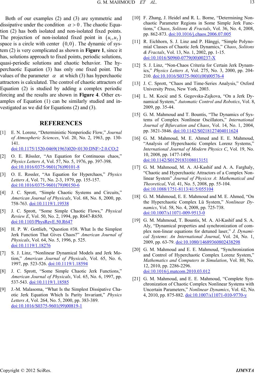

G. M. MAHMOUD ET AL. 13
Both of our exam and (3) are symmetric and
ive
ples (2)
dissipate under thcondition 0

.
ed fixed
The caotic Equa
tion (2) hasolated a
solat int in
h-
s both ind non-isolated fixed points.
The projection of non-ipo


,uu
12
space is a circle with center


0,0 . Tf sys-
tem (2) is very complicated as shown in Figure since it
has, solutions approach to fixed points, periodic solutions,
quasi-periodic solutions and chaotic behavior. The hy-
perchaotic Equation (3) has only one fixed point.
he dynami
1
va
c o
,
The
lues of the parameter

at which (3) has hyperchaotic
attractors is calculated. The control of chaotic attractors of
Equation (2) i by complex periodic
igure 4. Other ex-
s studied adding a
forcing and the results are shown in F
n (1) can be similarly studied and in
vestigated as we quations (2) an
REFERENCES
[1] E. N. Lorenz, “Deterministic Nonperiodic Flow,” Journal
of Atmospheric Sciences, Vol. 20, No. 2, 1963, pp. 130-
141.
doi:10.1175/1520-0469(1963)020<0130:DNF>2.0.CO;2
amples of Equatio-
did for Ed (3).
[2] O. E. Rössler, “An Equation for Continuous chaos,”
Physics Letters A, Vol. 57, No. 5, 1976, pp. 397-398.
doi:10.1016/0375-9601(76)90101-8
[3] O. E. Rossler, “An Equation for Hyperchaos,” Physics
Letters A, Vol. 71, No. 2-3, 1979, pp. 155-157.
doi:10.1016/0375-9601(79)90150-6
[4] J. C. Sprott, “Simple Chaotic Systems and Circuits,”
American Journal of Physicals, Vol. 68, No. 8, 2000, pp.
758-763. doi:10.1119/1.19538
[5] J. C. Sprott, “Some Simple Chaotic Flows,” Physical
Review E, Vol. 50, No. 2, 1994, pp. R647-R650.
doi:10.1103/PhysRevE.50.R647
[6] H. P. W. Gottlieb, “Question #38. What Is the Simplest
Jerk Function That Gives Chaos?” American Journal of
Physicals, Vol. 64, No. 5, 1996, p. 525.
doi:10.1119/1.18276
[7] S. J. Linz, “Nonlinear Dynamical Models and Jerk Mo-
tion,” American Journal of Physicals, Vol. 65, No. 6,
1997, pp. 523-526. doi:10.1119/1.18594
[8] J. C. Sprott, “Some Simple Chaotic Jerk Functions,”
American Journal of Physicals, Vol. 65, No. 6, 1997, pp.
537-543. doi:10.1119/1.18585
[9] J.-M. Malasoma, “What Is the Simplest Dissipative Cha-
otic Jerk Equation Which Is Parity Invariant,” Physics
Letters A, Vol. 264, No. 5, 2000, pp. 383-389.
doi:10.1016/S0375-9601(99)00819-1
Some Simple Je-
tions,” Chaons & Fractals l. 36, No. 008,
[10] F. Zhang, J. Heidel and R. L. Borne, “Determining Non-
chaotic Parameter Regions inrk Func
s, Solito, Vo4, 2
pp. 862-873. doi:10.1016/j.chaos.2006.07.005
[11] R. Eichhorn, S. J. Linz and P. Hänggi, “Simple Polyno-
mial Classes of Chaotic Jerk Dynamics,”litons
& Fractals, Vol. 13, No. 1, 2002, pp. 1-1
.1016/S0960-0779(00)002
Chaos, So
5.
doi:10 37-X
[12] S. J. Linz, “Non-Chaos Criteria for Certain Jerk Dynam-
ics,” Physics Letters A, Vol. 275, No. 3, 2000, pp. 204-
210. doi:10.1016/S0375-9601(00)00576-4
[13] J. C. Sprott, “Chaos and Time-Series Analysis,” Oxford
University Prerk, 2003.
[14] L. M. Kocić and S. Gegov
namical System,” Automatic Con
ss, New Yo
ska-Zajkova, “On a Jerk Dy-
trol and Robotics, Vol. 8,
2009, pp. 35-44.
5] G. M. Mahmoud and T. Bountis, “The Dynamics of Sys-
tems of Complex Nonlinear Oscillators,” International
Journal of Bifurcation and Chaos, Vol. 14, No. 1, 2004,
pp. 3821-3846. doi:10.1142/S0218127404011624
[1
[16] G. M. Mahmoud, M. E. Ahmed and E. E. Mahmoud,
“Analysis of Hyperchaotic Complex Lorenz Systems,”
International Journal of Modern Physics C, Vol. 19, No.
10, 2008, pp. 1477-1494.
doi:10.1142/S0129183108013151
[17] G. M. Mahmoud, M. A. Al-Kashif and A. A. Farghaly,
“Chaotic and Hyperchaotic Attractors of a Complex Non-
linear System” Journal of Physicss A: Mathematical and
Theoretical, Vol. 41, No. 5, 2008, pp. 55-104.
doi:10.1088/1751-8113/41/5/055104
[18] G. M. Mahmoud, E. E. Mahmoud and M. E. Ahmed, “On
the Hyperchaotic Complex Lü System,” Nonlinear Dy-
namics, Vol. 58, No. 4, 2008, pp. 725-738.
doi:10.1007/s11071-009-9513-0
[19] G. M. Mahmoud, T. Bountis, M. A. Al-Kashif and S. A.
Aly, “Dynamical properties and synchronization of com-
plex non-linear equations for detuned laser,” J. Dynami-
cal Systems: An International Journal, Vol. 24, No. 1,
2009, pp. 63-79. doi:10.1080/14689360802438298
[20] G. M. Mahmoud and E. E. Mahmoud, “Synchronization
and Control of Hyperchaotic Complex Lorenz System,”
Mathematics and Computers in Simulation, Vol. 80, No.
12, 2010, pp. 2286-2296.
doi:10.1016/j.matcom.2010.03.012
[21] G. M. Mahmoud, and E. E. Mahmoud, “Complete Syn-
chronization of Chaotic Complex Nonlinear Systems with
Uncertain Parameters,” Nonlinear Dynamics, Vol. 62, No.
4, 2010, pp. 875-882. doi:10.1007/s11071-010-9770-y