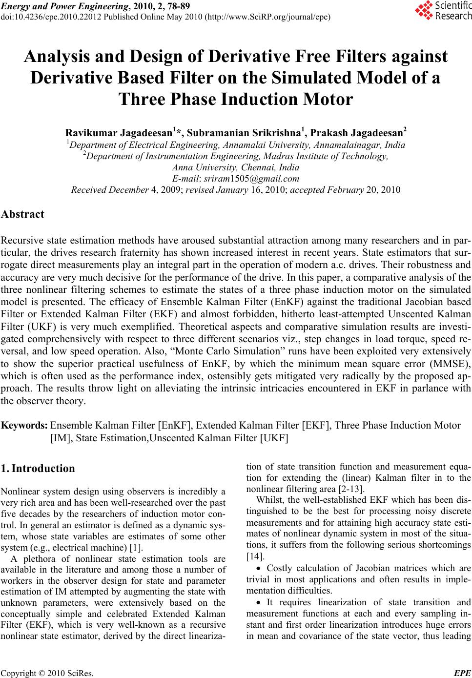Energy and Power Engineering, 2010, 2, 78-89
doi:10.4236/epe.2010.22012 Published Online May 2010 (http://www.SciRP.org/journal/epe)
Analysis and Design of Derivative Free Filters against
Derivative Based Filter on the Simulated Model of a
Three Phase Induction Motor
Ravikumar Jagadeesan1*, Subramanian Srikrishna1, Prakash Jagadeesan2
1Department of Electrical Engineering, Annamalai University, Annamalainagar, India
2Department of Instrumentation Engineering, Madras Institute of Technology,
Anna University, Chennai, India
Received December 4, 2009; revised January 16, 2010; accepted February 20, 2010
Abstract
Recursive state estimation methods have aroused substantial attraction among many researchers and in par-
ticular, the drives research fraternity has shown increased interest in recent years. State estimators that sur-
rogate direct measurements play an integral part in the operation of modern a.c. drives. Their robustness and
accuracy are very much decisive for the performance of the drive. In this paper, a comparative analysis of the
three nonlinear filtering schemes to estimate the states of a three phase induction motor on the simulated
model is presented. The efficacy of Ensemble Kalman Filter (EnKF) against the traditional Jacobian based
Filter or Extended Kalman Filter (EKF) and almost forbidden, hitherto least-attempted Unscented Kalman
Filter (UKF) is very much exemplified. Theoretical aspects and comparative simulation results are investi-
gated comprehensively with respect to three different scenarios viz., step changes in load torque, speed re-
versal, and low speed operation. Also, “Monte Carlo Simulation” runs have been exploited very extensively
to show the superior practical usefulness of EnKF, by which the minimum mean square error (MMSE),
which is often used as the performance index, ostensibly gets mitigated very radically by the proposed ap-
proach. The results throw light on alleviating the intrinsic intricacies encountered in EKF in parlance with
the observer theory.
Keywords: Ensemble Kalman Filter [EnKF], Extended Kalman Filter [EKF], Three Phase Induction Motor
[IM], State Estimation,Unscented Kalman Filter [UKF]
1. Introduction
Nonlinear system design using observers is incredibly a
very rich area and has been well-researched over the past
five decades by the researchers of induction motor con-
trol. In general an estimator is defined as a dynamic sys-
tem, whose state variables are estimates of some other
system (e.g., electrical machine) [1].
A plethora of nonlinear state estimation tools are
available in the literature and among those a number of
workers in the observer design for state and parameter
estimation of IM attempted by augmenting the state with
unknown parameters, were extensively based on the
conceptually simple and celebrated Extended Kalman
Filter (EKF), which is very well-known as a recursive
nonlinear state estimator, derived by the direct lineariza-
tion of state transition function and measurement equa-
tion for extending the (linear) Kalman filter in to the
nonlinear filtering area [2-13].
Whilst, the well-established EKF which has been dis-
tinguished to be the best for processing noisy discrete
measurements and for attaining high accuracy state esti-
mates of nonlinear dynamic system in most of the situa-
tions, it suffers from the following serious shortcomings
[14].
 Costly calculation of Jacobian matrices which are
trivial in most applications and often results in imple-
mentation difficulties.
 It requires linearization of state transition and
measurement functions at each and every sampling in-
stant and first order linearization introduces huge errors
in mean and covariance of the state vector, thus leading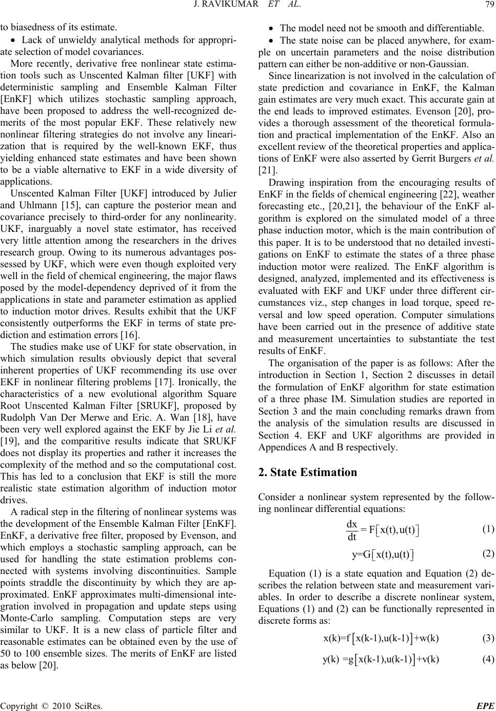

J. RAVIKUMAR ET AL.79
to biasedness of its estimate.
 Lack of unwieldy analytical methods for appropri-
ate selection of model covariances.
More recently, derivative free nonlinear state estima-
tion tools such as Unscented Kalman filter [UKF] with
deterministic sampling and Ensemble Kalman Filter
[EnKF] which utilizes stochastic sampling approach,
have been proposed to address the well-recognized de-
merits of the most popular EKF. These relatively new
nonlinear filtering strategies do not involve any lineari-
zation that is required by the well-known EKF, thus
yielding enhanced state estimates and have been shown
to be a viable alternative to EKF in a wide diversity of
applications.
Unscented Kalman Filter [UKF] introduced by Julier
and Uhlmann [15], can capture the posterior mean and
covariance precisely to third-order for any nonlinearity.
UKF, inarguably a novel state estimator, has received
very little attention among the researchers in the drives
research group. Owing to its numerous advantages pos-
sessed by UKF, which were even though exploited very
well in the field of chemical engineering, the major flaws
posed by the model-dependency deprived of it from the
applications in state and parameter estimation as applied
to induction motor drives. Results exhibit that the UKF
consistently outperforms the EKF in terms of state pre-
diction and estimation errors [16].
The studies make use of UKF for state observation, in
which simulation results obviously depict that several
inherent properties of UKF recommending its use over
EKF in nonlinear filtering problems [17]. Ironically, the
characteristics of a new evolutional algorithm Square
Root Unscented Kalman Filter [SRUKF], proposed by
Rudolph Van Der Merwe and Eric. A. Wan [18], have
been very well explored against the EKF by Jie Li et al.
[19], and the comparitive results indicate that SRUKF
does not display its properties and rather it increases the
complexity of the method and so the computational cost.
This has led to a conclusion that EKF is still the more
realistic state estimation algorithm of induction motor
drives.
A radical step in the filtering of nonlinear systems was
the development of the Ensemble Kalman Filter [EnKF].
EnKF, a derivative free filter, proposed by Evenson, and
which employs a stochastic sampling approach, can be
used for handling the state estimation problems con-
nected with systems involving discontinuities. Sample
points straddle the discontinuity by which they are ap-
proximated. EnKF approximates multi-dimensional inte-
gration involved in propagation and update steps using
Monte-Carlo sampling. Computation steps are very
similar to UKF. It is a new class of particle filter and
reasonable estimates can be obtained even by the use of
50 to 100 ensemble sizes. The merits of EnKF are listed
as below [20].
 The model need not be smooth and differentiable.
 The state noise can be placed anywhere, for exam-
ple on uncertain parameters and the noise distribution
pattern can either be non-additive or non-Gaussian.
Since linearization is not involved in the calculation of
state prediction and covariance in EnKF, the Kalman
gain estimates are very much exact. This accurate gain at
the end leads to improved estimates. Evenson [20], pro-
vides a thorough assessment of the theoretical formula-
tion and practical implementation of the EnKF. Also an
excellent review of the theoretical properties and applica-
tions of EnKF were also asserted by Gerrit Burgers et al.
[21].
Drawing inspiration from the encouraging results of
EnKF in the fields of chemical engineering [22], weather
forecasting etc., [20,21], the behaviour of the EnKF al-
gorithm is explored on the simulated model of a three
phase induction motor, which is the main contribution of
this paper. It is to be understood that no detailed investi-
gations on EnKF to estimate the states of a three phase
induction motor were realized. The EnKF algorithm is
designed, analyzed, implemented and its effectiveness is
evaluated with EKF and UKF under three different cir-
cumstances viz., step changes in load torque, speed re-
versal and low speed operation. Computer simulations
have been carried out in the presence of additive state
and measurement uncertainties to substantiate the test
results of EnKF.
The organisation of the paper is as follows: After the
introduction in Section 1, Section 2 discusses in detail
the formulation of EnKF algorithm for state estimation
of a three phase IM. Simulation studies are reported in
Section 3 and the main concluding remarks drawn from
the analysis of the simulation results are discussed in
Section 4. EKF and UKF algorithms are provided in
Appendices A and B respectively.
2. State Estimation
Consider a nonlinear system represented by the follow-
ing nonlinear differential equations:
dx =F x(t),u(t)
dt 
 
(1)
y=Gx(t),u(t)



 (2)
Equation (1) is a state equation and Equation (2) de-
scribes the relation between state and measurement vari-
ables. In order to describe a discrete nonlinear system,
Equations (1) and (2) can be functionally represented in
discrete forms as:


x(k)=fx(k-1),u(k-1)+w(k) (3)


y(k)=gx(k-1),u(k-1)+v(k) (4)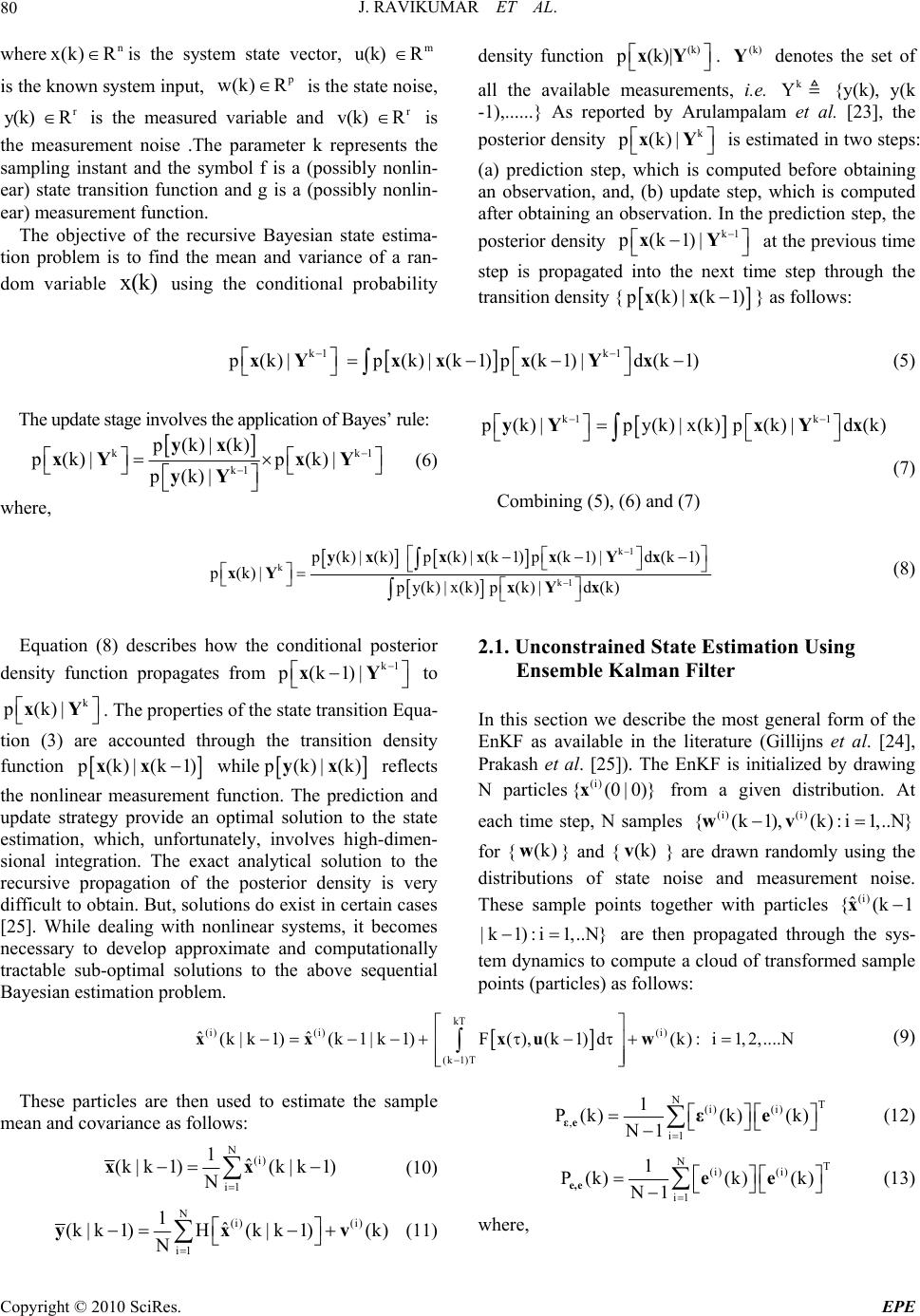

J. RAVIKUMAR ET AL. 80
where is the system state vector,
is the known system input,
n
x(k) Rm u(k) R
p
w(k) R is the state noise,
is the measured variable and is
the measurement noise .The parameter k represents the
sampling instant and the symbol f is a (possibly nonlin-
ear) state transition function and g is a (possibly nonlin-
ear) measurement function.
r
Ry(k) r k) Rv(
density function (k)
p(k)|




xY
k
p(k)|
. denotes the set of
all the available measurements, i.e. {y(k), y(k
-1),......} As reported by Arulampalam et al. [23], the
posterior density
(k)
Y
k
Y




xY
p(k1)|
is estimated in two steps:
(a) prediction step, which is computed before obtaining
an observation, and, (b) update step, which is computed
after obtaining an observation. In the prediction step, the
posterior density k1

 


Yx at the previous time
step is propagated into the next time step through the
transition density {


p(k)|(kxx1)} as follows:
The objective of the recursive Bayesian state estima-
tion problem is to find the mean and variance of a ran-
dom variable using the conditional probability
x(k)


k1 k1
p
(k) |p(k) |(k1)p(k1) |d(k1)

 

 

xYxxxY x

 (5)
The update stage involves the application of Bayes’ rule:


kk
k1
p(k)|(k)
p(k)| p(k)|
p(k)|


 

 


yx
xY xY
yY
1


(6)


k1 k1
p
(k) |py(k) | x(k)p(k) |d(k)

  
 

yYxY x
(7)
Combining (5), (6) and (7)
where,
 

k1
k
k1
p(k) |(k)p(k)|(k1)p(k1) |d(k1)
p(k)| py(k)|x(k)p(k)|d(k)




 




 



yxxxxY x
xY xY x
(8)
Equation (8) describes how the conditional posterior
density function propagates from to
. The properties of the state transition Equa-
tion (3) are accounted through the transition density
function
k1
p(k1)| 



xY
k
p(k)|


xY

2.1. Unconstrained State Estimation Using
Ensemble Kalman Filter



p(k)|(k1)xx while


p(k)|(k)yx reflects
the nonlinear measurement function. The prediction and
update strategy provide an optimal solution to the state
estimation, which, unfortunately, involves high-dimen-
sional integration. The exact analytical solution to the
recursive propagation of the posterior density is very
difficult to obtain. But, solutions do exist in certain cases
[25]. While dealing with nonlinear systems, it becomes
necessary to develop approximate and computationally
tractable sub-optimal solutions to the above sequential
Bayesian estimation problem.
In this section we describe the most general form of the
EnKF as available in the literature (Gillijns et al. [24],
Prakash et al. [25]). The EnKF is initialized by drawing
N particles from a given distribution. At
each time step, N samples
for {} and {} are drawn randomly using the
distributions of state noise and measurement noise.
These sample points together with particles
(i)
{(0|0)}x
(k) v
(i) (i)
{(k1),(k):i1,..N}wv
(i)
ˆ {(k1
(k)w

x
|k 1):i1,..N}

 are then propagated through the sys-
tem dynamics to compute a cloud of transformed sample
points (particles) as follows:

kT
(i) (i)(i)
(k 1)T
ˆˆ (k|k1)(k1|k1)F(),(k1)d(k):i 1,2,....N


  




xxxuw (9)
These particles are then used to estimate the sample
mean and covariance as follows:
NT
(i) (i)
,
i1
1
P (k)(k)(k)
N1


 


 

εeεe (12)
N(i)
i1
1ˆ
(k | k1)(k| k1)
N
 

xx (10) NT
(i) (i)
i1
1
P (k)(k)(k)
N1




e,e ee


(13)
N(i) (i)
i1
1ˆ
(k | k1)H(k | k1)(k)
N

 


yxv (11) where,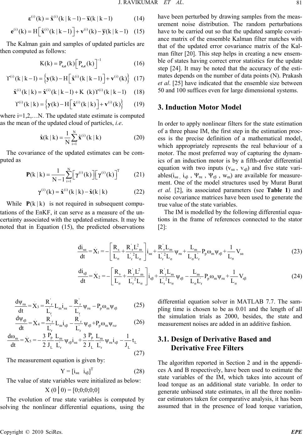

J. RAVIKUMAR ET AL.81
(i) (i)
ˆ
(k)(k|k 1)(k|k 1)εxx (14)
(i) (i)(i)
ˆ (k)H(k | k1)(k)(k | k1)



ex vy (15)
The Kalman gain and samples of updated particles are
then computed as follows:
1
K(k)P(k)P(k) 





ε,e e,e (16)


(i)(i) (i)
ˆ
(k | k1)(k)H(k| k1)(k)

 

yx v (17)
(i) (i)(i)
ˆˆ (k|k)(k|k 1)K(k)(k|k 1) xx  (18)


(i)(i) (i)
ˆ (k | k)(k)H(k | k)(k)

 

yx v (19)
where i=1,2,…N. The updated state estimate is computed
as the mean of the updated cloud of particles, i.e.
N(i)
i1
1
ˆˆ (k | k)(k | k)
N
 xx (20)
The covariance of the updated estimates can be com-
puted as
NT
(i) (i)
i1
1
(k | k)(k)(k)
N1




Pγγ


(21)
(i) (i)
ˆˆ
(k)(k |k)(k | k)γxx (22)
While is not required in subsequent compu-
tations of the EnKF, it can serve as a measure of the un-
certainty associated with the updated estimates. It may be
noted that in Equation (15), the predicted observations
(k | k)P
have been perturbed by drawing samples from the meas-
urement noise distribution. The random perturbations
have to be carried out so that the updated sample covari-
ance matrix of the ensemble Kalman filter matches with
that of the updated error covariance matrix of the Kal-
man filter [20]. This step helps in creating a new ensem-
ble of states having correct error statistics for the update
step [24]. It may be noted that the accuracy of the esti-
mates depends on the number of data points (N). Prakash
et al. [25] have indicated that the ensemble size between
50 and 100 suffices even for large dimensional systems.
3. Induction Motor Model
In order to apply nonlinear filters for the state estimation
of a three phase IM, the first step in the estimation proc-
ess is the precise definition of a mathematical model,
which appropriately represents the real behaviour of a
motor. The most preferred way of capturing the dynam-
ics of an induction motor is by a fifth-order differential
equation with two inputs (vsα , vsβ) and five state vari-
ables(isα , i
sβ , Ψrα , Ψrβ , wm) are available for measure-
ment. One of the model structures used by Murat Burat
et al. [2], its associated parameters (see Table 1) and
noise covariance matrices have been used to generate the
true value of the state variables.
The IM is modelled by the following differential equa-
tions in the frame of references connected to the stator
[2]:
'2 '
.
sαsrm rmm
1sαrαpmrβsα
'2 '2'
σσ rσrσσr
diR RL RLL1
=X =+i+ψ+Pωψ+V
dt LL LLLL LL


 (23)
'2 '
.
sβsrm rmm
2sβrβpmrαsβ
'2'2'
σσ rσrσσr
di RRL RLL1
=X =+i+ψPωψ+V
dt LL
LLLL LL



 (24)
''
.
rαrr
3msαrαpmrβ
''
rr
dψRR
=X =L iψPωψ
dt LL
 (25)
''
.
rβrr
4msβrβ
p
mr
''
rr
dψRR
=X=L iψ+P ωψ
dt LL

 (26)
.pp
mmm
5rβsαrαsβL
''
LL rr
PP
dωLL 33
=X =ψi+ ψit
dt 2J2JJ LL

L
1

(27)
The measurement equation is given by:
Y = [isα isβ]T (28)
The value of state variables were initialized as below:
X (0│0) = [0;0;0;0;0]
The evolution of true state variables is computed by
solving the nonlinear differential equations, using the
differential equation solver in MATLAB 7.7. The sam-
pling time is chosen to be as 0.01 and the length of all
the simulation trials as 2000, besides, the state and
measurement noises are added in an additive fashion.
3.1. Design of Derivative Based and
Derivative Free Filters
The algorithm reported in Section 2 and in the appendi-
ces A and B respectively, have been used to estimate the
state variables of the IM, which takes into account of
load torque as an additional state variable. In order to
generate unbiased state estimates, in all the three nonlin-
ear estimators taken for comparative analysis, it has been
assumed that in the presence of load torque variation,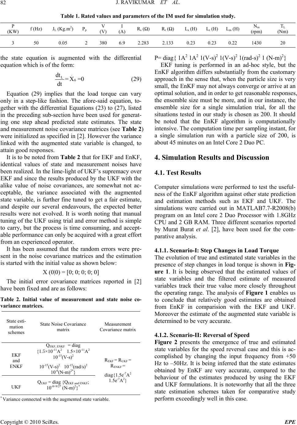

J. RAVIKUMAR ET AL. 82
Table 1. Rated values and parameters of the IM used for simulation study.
P
(KW) f (Hz) JL (Kg.m2) Pp
V
(V)
I
(A) Rs (Ω) Rr (Ω) Ls (H)Lr (H)Lm (H) Nm (rpm)
TL
(Nm)
3 50 0.05 2 380 6.9 2.283 2.133 0.23 0.23 0.22 1430 20
the state equation is augmented with the differential
equation which is of the form:
.
L6
dt =X =0
dt (29)
Equation (29) implies that the load torque can vary
only in a step-like fashion. The afore-said equation, to-
gether with the differential Equations (23) to (27), listed
in the preceding sub-section have been used for generat-
ing one step ahead predicted state estimates. The state
and measurement noise covariance matrices (see Table 2)
were initialized as specified in [2]. However the variance
linked with the augmented state variable is changed, to
attain good responses.
It is to be noted from Table 2 that for EKF and EnKF,
identical values of state and measurement noises have
been realized. In the lime-light of UKF’s supremacy over
EKF and since the results produced by the UKF with the
alike value of noise covariances, are somewhat not ac-
ceptable, the variance associated with the augmented
state variable, is further fine tuned to get a fair estimate,
and despite our several endeavours, the expected better
results were not evolved. It is worth noting that manual
tuning of the UKF using trial and error method is simple
to carry, but the process is time consuming, and accept-
able performance can only be acquired with a great effort
from an experienced operator.
It has been assumed that the random errors were pre-
sent in the noise covariance matrices and the estimation
is started with the initial value as shown below:
X (0|0) = [0; 0; 0; 0; 0]
The initial error covariance matrices reported in [2]
have been fixed and are as follows:
Table 2. Initial value of measurement and state noise co-
variance matrices.
State esti-
mation
schemes
State Noise Covariance
matrix
Measurement
Covariance matrix
EKF
and
ENKF
QEKF, ENKF = diag
{1.5×10-11A2 1.5×10-11A2
10-15(V-s)2
10-15(V-s)2 10-15(rad/s)2
10-6(N-m)2*}
UKF
QUKF = diag {QEKF and ENKF;
10-8+9/2 * (N-m)2}*
REKF = RUKF =
RENKF =
diag{1.5e-7A2
1.5e-7A2}
* Variance connected with the augmented state variable.
P= diag{ 1A2 1A2 1(V-s)2 1(V-s)2 1(rad-s)2 1 (N-m)2}
EKF tuning is performed in an ad-hoc style, but the
EnKF algorithm differs substantially from the customary
approach in the sense that, when the particle size is very
small, the EnKF may not always converge or arrive at an
optimal solution, and in order to get reasonable responses,
the ensemble size must be more, and in our instance, the
ensemble size for a single simulation trial, for all the
situations tested in our study is chosen as 200. It should
be noted that the EnKF algorithm is computationally
intensive. The computation time per sampling instant, for
a single simulation run with a particle size of 200, is
about 45 minutes on an Intel Core 2 Duo PC.
4. Simulation Results and Discussion
4.1. Test Results
Computer simulations were performed to test the useful-
ness of the EnKF algorithm against other state prediction
and estimation methods such as EKF and UKF. The
simulations were carried out in MATLAB7.7-R2008(b)
program on an Intel core 2 Duo Processor with 1.8GHz
CPU and 2 GB RAM. Three different scenarios reported
by Murat Burat et al. [2], have been used for the com-
parative analysis.
4.1.1. Scenario-I: Step Changes in Load Torque
The evolution of true and estimated state variables in the
presence of step changes in load torque is shown in Fig-
ure 1. It is being observed that the estimated values of
state variables and the filtered estimate of measured
variables track their true value more closely throughout
the operating range. The analysis of Figure 1 enables us
to conclude that relatively good estimates are obtained
from EnKF in comparision with the EKF and UKF.
Moreover the estimate of the augmented state variable is
determined to be very accurate.
4.1.2. Scenario-II: Reversal of Speed
Figure 2 presents the emergence of true and estimated
state variables for the speed reversal case and this is ac-
complished by changing the input frequency from +50
Hz to –50Hz. It is being inferred that the state estimates
obtained by EnKF are very accurate, compared to the
behaviour of the estimates produced by using the EKF
and UKF formulations. It is noteworthy that all the three
state estimation schemes taken for comparative study
perform exceedingly well in this case.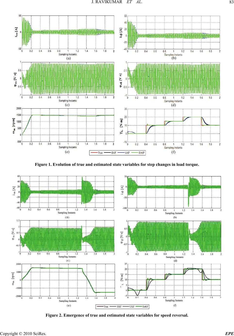

J. RAVIKUMAR ET AL. 83
2
Figure 1. Evolution of true and estimated state variables for step changes in load torque.
Figure 2. Emergence of true and estimated state variables for speed reversal.
(d)
(c)
(e) (f)
(b)
(a)
2
2
C
opyright © 2010 SciRes. EPE

J. RAVIKUMAR ET AL. 84
4.1.3. Scenario-III: Low Speed Operation
One significant aspect being very well examined in the
literature is the low speed operation, which was pre-
sumed as a serious challenge in the arena of IM drives.
This is possible by constantly maintaining v/f ratio and
the low speed operation results are very well displayed in
Figure 3. A closer examination of the Figure 3 discloses
that the estimates of speed and rotor fluxes are found to
be more precise. It should be noted that the Kalman filter
and its variants have demonstrated an acceptable per-
formance in the low speed operation. Regardless of its
appreciable results of simulation at low speeds for EKF
algorithm, the complexity, computational burden and
accuracy issues practically outlaw the choice of EKF
algorithm over a low-cost fixed processor.
a) isα[A]-Stator stationary axis components of stator
currents. b) isβ[A]-Stator stationary axis components of
stator currents. c) -Rotor stationary axis compo-
nents of stator flux. d) -Rotor stationary axis
components of stator flux. e) ωm [rad-s]-Angular velocity.
f) TL[N-m]-Load torque.
rα
ψ[V-s]
rβ
ψ[V-s]
4.2. Performance Assessment
The performance of the three nonlinear estimators taken
for comparative study must be assessed through simula-
tion, because stochastic systems are involved in these
studies. For each case that is being analyzed, a simula-
tion run that consists of NT (trials) with the length of
each simulation trial being equal to L is conducted. In all
the simulation trials, the sum of the squares of the esti-
mation errors, which is truly the difference between the
estimated value of the state variables and the true value
of the state variables, that have been obtained. The mean
of the estimation errors based on 25 Monte Carlo simula-
tions for the EKF, UKF and ENKF are reported in Ta-
bles 4, 5 and 6 respectively. A close view at the tables
makes one to conclude that, the Minimum Mean Square
Error [MMSE], which is often used as a performance
index is found to be very low for EnKF in all the three
different scenarios taken for comparative simulation
study. It is apparent from the Table 6 that, MMSE gets
lessened by the use of more ensemble sizes. The compu-
tational time per sampling instant for an ensemble size of
25 for EnKF is compared with the EKF and UKF and
presented in the form of histogram (see Figure 4). De-
spite the fact that the time-complexity is said to be large,
these are well within the capabilities of contemporary
signal processing devices, so that a real-time accom-
plishment is plausible.
5. Concluding Remarks
An attempt has been made in this paper to use the EnKF
for the estimation of states of a three phase IM. Computer
simulations have been performed meticulously to
Figure 3. Emergence of true and estimated state variables for low speed operation.
C
opyright © 2010 SciRes. EPE

J. RAVIKUMAR ET AL.85
Figure 4. Comparision of execution time of EnKF for a particle size 25 against EKF and UKF.
Table 4. Minimum mean square error (MMSE) values of
EKF.
SCENARIO –
I
SCENARIO –
II
SCENARIO –
III
STATE
VARI-
ABLES MEAN MEAN MEAN
sα
i 6.9100e-2 6.6720e-2 1.8400e-2
sβ
i 6.9093e-2 6.6723e-2 1.8469e-2
rα
ψ 6.0288e-5 5.8286e-5 1.1682e-4
rβ
ψ 6.0290e-5 5.8282e-5 1.3016e-4
m
ω 9.4296e-1 9.7334e-1 4.8508e-1
L
t 5.5802e0 5.5872e0 2.0452e0
Table 5. Minimum mean square error (MMSE) values of
UKF.
SCENARIO –
I
SCENARIO –
II
SCENARIO –
III
STATE
VARI-
ABLES MEAN MEAN MEAN
sα
i 1.8604e-1 2.6480e-1 3.1616e-1
sβ
i 1.8611e-1 2.6479e-1 3.0686e-1
rα
ψ 1.0164e-4 1.4123e-4 1.8700e-3
rβ
ψ 1.0357e-4 1.4314e-4 2.2864e-3
m
ω 1.1745e0 2.1488e0 2.3092e0
L
t 4.6709e0 4.7167e0 2.6369e0
compare the behaviour of EnKF against the EKF and
UKF. The main conclusion drawn from this work, is that
the inherent flaw of the well-appreciated EKF i.e., the
exhaustive Jacobian computation, which is very well the
cause of biasedness of its estimate and imposing severe
computational cost in real-time implementation were
overcome, thanks to the action of EnKF, which provides
a derivative free approach for estimation of predicted
covariances required in the update step. As evidenced by
the results, the EnKF algorithm surpasses EKF and UKF
in all the scenarios tested, and a noticeable enhancement
in its performance is attained even by the use of 50 to
100 ensemble sizes. This can be claimed as a potential
advantage over EKF.
Enlightened by the belief that UKF is a superior alter-
native of the EKF, though theoretically proven, it is fine
tuned to obtain an estimate very nearer to EKF, but even
then UKF did not exhibit its properties, and the results
achieved are said to be implausible. Additive and Gaus-
sian noise distribution sequence is usually made as an
assumption in the state estimation of a three phase IM.
However, there are schools of thought supporting the
distribution of noise in IM drive system in real-time, as
being primarily non-addditive and non-Gaussian in na-
ture. Categorically, the drives research community has
been left bewildered by such an apparent dissension and
even under such circumstances, the EnKF algorithm will
work satisfactorily, which has to be further explored
carefully. Conversely, the well-acclaimed EKF can be
strictly applied only for restricted class of noise distribu-
tion patterns. Because of its conspicuous performance,
the EnKF algorithm has an edge over EKF in a wide di-
versity of applications. The only drawback is the
time-complexity, but nevertheless a processor with high

J. RAVIKUMAR ET AL. 86
Table 6. Minimum mean square Error (MMSE) values of EnKF for different ensemble sizes.
PARTICLE SIZE STATE VARIABLES SCENARIO I SCENARIO II SCENARIO III
sα
i 7.2293e-4 5.5775e-4 1.1594e-4
sβ
i 7.2395e-4 5.5142e-4 1.8477e-4
rα
ψ 2.3036e-5 2.7246e-5 2.7319e-5
rβ
ψ 1.9797e-5 2.0483e-5 2.0248e-5
m
ω 3.2161e-2 2.5811e-2 1.9117e-2
25
L
t 1.4886e0 1.3837e0 5.0224e-1
sα
i 5.3629e-4 4.3726e-4 8.0065e-5
sβ
i 5.4094e-4 4.3459e-4 1.5401e-4
rα
ψ 1.3467e-5 1.7553e-5 1.7393e-5
rβ
ψ 9.0231e-6 8.8537e-6 8.6287e-6
m
ω 2.8156e-2 2.3189e-2 1.7070e-2
50
L
t 1.4234e0 1.3300e0 4.8683e-1
sα
i 4.5133e-4 3.8873e-4 7.7783e-5
sβ
i 4.5348e-4 3.8735e-4 1.4255e-4
rα
ψ 1.2643e-5 1.7070e-5 1.7924e-5
rβ
ψ 7.7786e-6 7.4994e-6 7.2875e-6
m
ω 2.6420e-2 2.2476e-2 1.5958e-2
75
L
t 1.3917e0 1.3212e0 4.7789e-1
sα
i 4.5836e-4 3.8299e-4 7.0702e-5
sβ
i 4.5023e-4 3.8734e-4 1.3433e-4
rα
ψ 9.6340e-6 1.3041e-5 1.6903e-5
rβ
ψ 6.5697e-6 6.3207e-6 6.1035e-6
m
ω 2.6116e-2 2.1808e-2 1.5007e-2
100
L
t 1.4050e0 1.3219e0 4.8265e-1
sα
i 4.2953e-4 3.5544e-4 6.8404e-5
sβ
i 4.4175e-4 3.6098e-4 1.2849e-4
rα
ψ 1.1029e-6 1.5337e-5 1.5158e-5
rβ
ψ 2.4206e-6 2.0697e-6 1.8484e-6
m
ω 2.5491e-2 2.2614e-2 1.4785e-2
150
L
t 1.3995e0 1.3059e0 4.7555e-1
calculation performance can accomplish these require
ments. Since the digitized a.c. drives have reached the
state-of-the-art of technology, any order of these chal-
lenging crossroads can be proven to be mediocre.
6
. References
[1] P. Vas, “Sensorless Vector and Direct Torque Control,”
Oxford University Press, New York, 1998.
C
opyright © 2010 SciRes. EPE

J. RAVIKUMAR ET AL.87
[2] M. Burat, S. Bogosyan and M. Gokasan, “Speed Sensor-
less Estimation for Induction Motors Using Extended
Kalman Filters,” IEEE Transactions on Industrial Elec-
tronics, Vol. 54, No. 1, February 2007, pp. 272-280.
[3] M. Burat, S. Bogosyan and M. Gokasan, “Braided Ex-
tended Kalman Filters for Sensorless Estimation in In-
duction Motors at High-low/Zero Speed,” IET Control
Theory & Applications, Vol. 1, No. 4, 2007, pp. 987-998.
[4] M. Burat, S. Bogosyan and M. Gokasan, “Speed Sensor-
less Direct Torque Control of IMs with Rotor Resistance
Estimation,” Energy Conversion and Management, Vol.
46, No. 3, 2005, pp. 335-349.
[5] M. Burat, S. Bogosyan and M. Gokasan, “An EKF Based
Estimator for Speed Sensorless Vector Control of Induc-
tion Motors,” Electric Power Components and Systems,
Vol. 33, No. 7, 2005, pp. 727-744.
[6] J. Holtz, “Sensorless Control of Induction Machines with
or without Signal Injection?” IEEE Transactions on In-
dustrial Electronics, Vol. 53, No. 1, February 2006, pp.
7-30.
[7] J. W. Finch, D. J. Atkinson and P. P. Acarnley, “Full-
Order Estimator for Induction Motor States and Parame-
ters,” IEE Electric Power Applications, Vol. 145, No. 3,
May 1998, pp. 169-179.
[8] C. Lascu, I. Boldea and F. Blaabjerg, “Comparitive Study
of Adaptive and Inherently Sensorless Observers for
Variable Speed Induction Motor Drives,” IEEE Transac-
tions on Industrial Electronics, Vol. 53, No. 1, February
2006, pp. 57-65.
[9] G. G. Soto, E. Mendes and A. Razek, “Reduced-Order
Observers for Rotor Flux, Rotor Resistance and Speed
Estimation for Vector Controlled Induction Motor Drive
Using the Extended Kalman Filter Technique,” IEE Pro-
ceedings Electric Power Applications, Vol. 146, No. 3,
May 1999.
[10] H.-W. Kim and S.-K. Sul, “A New Motor Speed Estima-
tor Using Kalman Filter in Low-Speed Range,” IEEE
Transactions on Industrial Electronics, Vol. 43, No. 4,
August 1996, pp. 498-504.
[11] D. J. Atkinson, J. W. Finch and P. P. Acarnley, “Estima-
tion of Rotor Resistance in Induction Motors,” IEE Pro-
ceedings Electric Power Applications, Vol. 146, No. 3,
January 1996.
[12] K. L. Shi, T. F. Chan, Y. K. Wong and S. L. Ho, “Speed
Sensorless Control of an Induction Motor Drive Using an
Optimized Extended Kalman Filter,” IEEE Transactions
on Industrial Electronics, Vol. 49, No. 1, February 2002,
pp. 124-133.
[13] Y.-R. Kim, S.-K. Sul and M.-H. Park, “Speed Sensorless
Vector Control of Induction Motor Using Extended Kal-
man Filter,” IEEE Transactions on Industrial Electronics,
Vol. 30, No. 5, September/October 1994, pp. 1225-1233.
[14] S. Julier, J. K. Uhlmann and H. F. Durrant-Whyte, “A
New Method for the Nonlinear Transformation of Means
and Covariances in Filters and Estimators,” IEEE Trans-
actions on Automatic Control, Vol. 45, No. 3, March
2000, pp. 477-482.
[15] S. J. Julier and J. K. Uhlmann, “Unscented Filtering and
Nonlinear Estimation,” Proceedings of the IEEE, Vol. 92,
No. 3, March 2004, pp. 401-422.
[16] K. Xiong, H. Y. Zhang and C. W. Chan, “Performance
Evaluation of UKF-Based Nonlinear Filtering,” Auto-
matica, Vol. 42, 2006, pp. 261-270.
[17] B. Akin, U. Orguner and A. Ersak, “State Estimation
Using Unscented Kalman Filter,” Proceedings of IEEE,
2003, pp. 915-919.
[18] R. van der Merwe and E. A. Wan, “The Square-Root
Unscented Kalman Filter for State and Parameter Estima-
tion,” Proceedings of the International Conference on
Acoustics, Speech and Signal Processing, May 2001.
[19] J. Lie, Y. R. Zhong and H. P. Ren, “Speed Estimation of
Induction Machines Using Square Root Unscented Kal-
man Filter,” Proceedings of the IEEE, 2005, pp. 674-679.
[20] G. Evensen, “Ensemble Kalman Filter: Theoretical For-
mulation and Practical Implementation,” Ocean Dynam-
ics, Vol. 53, 2003, pp. 343-367.
[21] G. Burgers, P. J. Van Leeuwen and G. Evenson, “Analy-
sis Scheme in Ensemble Kalman Filter,” American Mete-
orological Society, Vol. 126, 1998, pp. 1719-1724.
[22] J. Prakash, S. C. Patwardhan and S. L. Shah, “Constrain-
ed State Estimation Using the Ensemble Kalman Filter,”
Proceedings of the American Control Conference, 2008,
pp. 3542-3547.
[23] M. S. Arulampalam, S. Maskell, N. Gordon and T. Clapp,
“A Tutorial on Particle Filters for Online Nonlinear/Non-
Gaussian Bayesian Tracking,” IEEE Transactions on
Signal Processing, Vol. 50, No. 2, 2002, pp. 174-188.
[24] S. Gillijns, O. B. Mendoza, J. Chandrasekar, B. L. R. De
Moor, D. S. Bernstein and A. Ridley, “What is the En-
semble Kalman Filter and How Well does it Work?”
Proceedings of the American Control Conference, 2006,
pp. 4448-4453.
[25] S. C. Patwardhan, J. Prakash and S. L. Shah, “Soft Sens-
ing and State Estimation: Review and Recent Trends,”
Proceedings of IFAC Conference on Cost Effective
Automation, Mexico, Vol. 1, Part 1, 2008.

J. RAVIKUMAR ET AL. 88
Nomenclature
Pp No. of pole pairs
σs
L=σL Stator transient inductance (H)
σ Leakage or Coupling factor
Ls Stator inductance (H)
Rs Stator resistance (Ω)
'
r
L Rotor inductance referred to the stator
side (Ω)
'
r
R Rotor resistance referred to the stator side
(Ω)
sα
V, sβ V Stator stationary axis components of
stator currents (V)
rαrβ
ψ,ψ Rotor stationary axis components of
stator flux (V-s)
L
J Total inertia of the IM (Kg.m2)
m
ω Angular velocity
x True state variables
ˆ
x(k | k) Updated state estimates
y(k) Measured variables
u(k) Input variables
P(k | k) Updated error covariance matrix
W(k) State noise vectors
F Jacobian matrix
G Non linear measurement function
ˆ
x(k | k1)
 Predicted state estimates
P(k | k1) Predicted error covariance matrix
ˆ
y(k | k1)
 Predicted measurement
(k | k1) Innovation matrix
K(k) Kalman gain
V(k) Covariance matrix of innovation
(k | k,i)

A set of 2L+I sigma points
(k | k1,i)

 Predicted set of sigma points
ee
P(k) Covariance matrix of innovations
e
P(k)

Cross covariance matrix between the
predicted state estimate errors and
innovations
W(i) Associated weights
Greek Symbols
Ф State transition matrix
µ Mean of estimation error
Appendix-A
EKF Algorithm
Owing to a wealth of literature exists on the EKF algo-
rithm, here we merely present the filter equation in a
succinct way. The basic idea of the EKF is to linearize f
and g (Equations (3) and (4) listed in the Section 2) using
a first order Taylor series expansion, and then apply the
standard Kalman filter. We have assumed in this work
that the initial state and the sequence 

w(k) and


v(k)
are white, Gaussian and independent of each other. The
most acclaimed EKF is as follows:
The predicted state estimates are obtained as:

(k)T
(k 1)T
ˆˆ (k|k 1)(k1|k1)F(),(k 1)d


 

xx xu
(A.1)
The covariance matrix of estimation errors in the pre-
dicted estimates is obtained as
T
P(k|k1)(k)P(k1|k1)(k) Q  (A.2)
where
 

ˆˆ x ( k1|k1),u ( k1)x ( k1|k1),u ( k1)
FG
A(k) ;C(k)
xx
(k)exp A(k)*T
 

 

 

 

(k)

is nothing but Jacobian matrices of partial de-
rivatives of


F. with respect to x and w and is
the Jacobian matrix of partial derivatives of
C(k)


H. with
respect to x. The measurement prediction, computation
of innovation and covariance matrix of innovation are as
follows:


ˆˆ
y(k|k 1)Hx(k|k 1)

 (A.3)
ˆ (k | k1)y(k)y(k | k1)

  (A.4)
T
V(k)C(k)P(k | k1)C(k)R

 (A.5)
The Kalman gain is computed using the following
equation
T1
K(k)P(k | k1)C(k)V(k)

 (A.6)
The updated state estimates are obtained using the
following equation
ˆˆ
x(k | k)x(k | k1)K(k)(k | k1)

   (A.7)
The covariance matrix of estimation errors in the up-
dated state estimates is obtained as


P(k | k)IK(k)C(k)P(k |k1)

 (A.8)
It should be noted that the calculation of the covari-
ances and the gain of the EKF are the same as those of
the linear Kalman filter. The EKF always approximates
k
p
x(k)| Y



 to be Gaussian. However, the distribu-

J. RAVIKUMAR ET AL. 89
tions of the various random variables are no longer nor-
mal after undergoing their respective nonlinear transfor-
mations. Moreover, EKF uses first order terms of the
Taylor series expansion of the nonlinear functions, so,
large errors will be introduced when the models are
highly nonlinear.
Appendix-B
Unscented Kalman Filter Algorithm (Julier and
Uhlmann, 2000)
The unscented transformation (UT) is a method for cal-
culating the statistics of a random variable, which un-
dergoes a nonlinear transformation. A set of 2L+1 sigma
points (k | k,i)

with the associated weights are
chosen symmetrically about as follows:
W(i)
ˆ
x(k | k)
0
ˆ
(k | k,0)x(k | k)WL

 



i
ˆ
(k |k,i)x(k / k)(L)P(k | k)
1
W(i)i1: L
2(L )
 




iL
ˆ (k|k,i)x(k|k)(L)P(k|k)
1
W(i); iL1.....2L
2(L )




where is a tuning parameter and for Gaussian distri-
bution the tuning parameter can be obtained from the
following relation . The 2L+1 sigma points
have been derived from the state () and covari-
ance of the state vector (), where L is the dimen-
sion of the state.

3L 
P(k |
ˆ
x(k | k)
k )
In the prediction step, the sigma points are propagated
through the nonlinear differential equations to obtain the
predicted set of sigma points as

kT
(k 1)T
(k|k 1,i)(k 1|k 1,i)F(,i),(k 1)
d;i0:2L

 

u

(B.1)
The predicted state estimates () are ob-
tained from the predicted sigma points as
ˆ
x(k | k1)
2L
i0
ˆ x(k|k1)W(i)(k|k1,i)

 
 (B.2)
The error covariance matrix (P( ) is obtained
from the predicted sigma points as
k | k1)
2L
i0
T
ˆ
P(k|k1) W(i)[(k|k1,i)x(k/k1)]
ˆ
[(k|k 1,i)x(k/k 1)]Q



 
 (B.3)
The predicted sigma points are propagated through the
nonlinear measurement equation to obtain the predicted
measurement as
(B.4)

2L
i0
ˆ
y(k|k 1)W(i)*H(k|k 1,i)

 

The covariance matrix of the innovations () and
the cross covariance matrix between the predicted state
estimate errors and innovations () are computed
as:
ee
P(k)
e
P(k)

2L
ee
i0
T
P(k)W(i){H[(k|k 1,i)]
ˆˆ
y(k | k1)}*{H[(k | k1,i)]y(k | k1)}


 
 (B.5)
2L
e
i0
T
P(k)W(i)[(k|k1,i)
ˆˆ
x(k/ k1)]*{H[(k | k1,i)]y(k | k1)}


 
 (B.6)
ˆ (k | k1)y(k)y(k |k1)

  (B.7)
The Kalman gain matrix () can be determined as
follows:
K(k)
1
eee
K(k)P (k)P(k)


 (B.8)
The updated state estimates () are obtained
using the linear update equation as in the Kalman filter.
ˆ x(k | k)
ˆˆ
x(k | k)x(k | k-1)K(k)|(k | k-1)

 (B.9)
The covariance matrix of error in the updated state es-
timates () are computed using P(k | k)
T
ee
P(k | k)P(k | k-1)-K(k)*P(k)K(k) (B.10)
The UKF does not approximate the nonlinear func-
tions of system and measurement models as required by
the EKF. Instead, the nonlinear functions are applied to
sigma points to yield transformed samples, and the
propagated mean and covariance are calculated from the
transformed samples.