Paper Menu >>
Journal Menu >>
 Open Journal of Fluid Dynamics, 2012, 2, 1-13 http://dx.doi.org/10.4236/ojfd.2012.21001 Published Online March 2012 (http://www.SciRP.org/journal/ojfd) 1 Effects of Hall Current and Ion-Slip on Unsteady MHD Couette Flow Nirmal Ghara, Sovan Lal Maji, Sanatan Das, Rabindranath Jana1, Swapan Kumar Ghosh2 1Department of Applied Mathematics, Vidyasagar University, Midnapore, India 2Department of Mathematics, Narajole Raj College, Narajole, India Email: jana261171@yahoo.co.in, g_swapan2002@yahoo.com Received November 26, 2011; revised December 15, 2011; accepted December 28, 2011 ABSTRACT The unsteady MHD Couette flow of an incompressible viscous electrically conducting fluid between two infinite non- conducting horizontal porous plates under the boundary layer approximations has been studied with the consideration of both Hall currents and ion-slip. An analytical solution of the governing equations describing the flow is obtained by the Laplace transform method. It is seen that the primary velocity decreases while the magnitude of secondary velocity in- creases with increase in Hall parameter. It is also seen that both the primary velocity and the magnitude of secondary velocity decrease with increase in ion-slip parameter. It is observed that a thin boundary layer is formed near the sta- tionary plate for large values of squared Hartmann number and Reynolds number. The thickness of this boundary layer increases with increase in either Hall parameter or ion-slip parameter. Keywords: MHD; Couette Flow; Porous Plate; Hall Current; Ion-Slip; Hartmann Number and Reynolds Number 1. Introduction The magnetohydrodynamic (MHD) flow between two parallel plates, one in uniform motion and the other held at rest known as MHD Couette flow, is a classical prob- lem that has many applications in MHD power genera- tors and pumps, accelerators, aerodynamic heating, elec- trostatic precipitation, polymer technology, petroleum industry, purification of crude oil and fluid droplets and sprays. A lot of research work concerning the MHD Couette flow has been obtained under different physical effects. In most cases, the Hall and ion slip terms were ignored in applying Ohm's law as they have no marked effect for small and moderate values of the magnetic field. However, the current trend for the application of magnetohydrodynamics is towards a strong magnetic field, so that the influence of electromagnetic force is noticeable [1]. Under these conditions, the Hall currents and ion slip are important and they have a marked effect on the magnitude and direction of the current density and consequently on the magnetic force term. Soundalgekar [2] has studied the Hall and ion-slip effects in MHD Coutte flow with heat transfer. Attia [3] has studied the unsteady Couette flow with heat transfer considering ion- slip. The transient Hartmann flow with heat transfer con- sidering the ion slip has been investigated by Attia [4-6]. Attia [7] has obtained the analytical solution for flow of a dusty fluid in a circular pipe with Hall and ion slip effect. Seddeek [8] has studied the effects of Hall and ion-slip currents on magneto-micropolar fluid and heat transfer over a non-isothermal stretching sheet with suction and blowing. The effects of Hall and ion-slip currents on free convective heat generating flow in a rotating fluid have studied by Ram [9]. Mittal and Bhat [10] has discussed the forced convective heat transfer in a MHD channel with Hall and ion slip currents. Jana and Datta [11] has described the Couette flow and heat transfer in a rotating system. The Hall effect on unsteady Couette flow under boundary layer approximations has been analysed by Kanch and Jana [12]. Attia [13] has studied the ion slip effect on unsteady Couette flow with heat transfer under exponential decaying pressure gradient. The combined effect of Hall and ion-slip currents on unsteady MHD Couette flows in a rotating system have been investigated by Jha and Apere [14]. The present paper is devoted to study the combined effects of Hall current and ion-slip on the unsteady MHD Couette flow between two infinite horizontal parallel porous plates under the boundary layer approximations. The upper plate is moving with a uniform velocity U while the lower plate is held at rest. The fluid is acted upon by a constant pressure gradient and a uniform suc- tion/injection at the plates. A uniform magnetic field 0 is applied perpendicular to the plates. It is found that the primary velocity decreases while the magnitude of the secondary velocity increases with increase in Hall pa- B C opyright © 2012 SciRes. OJFD 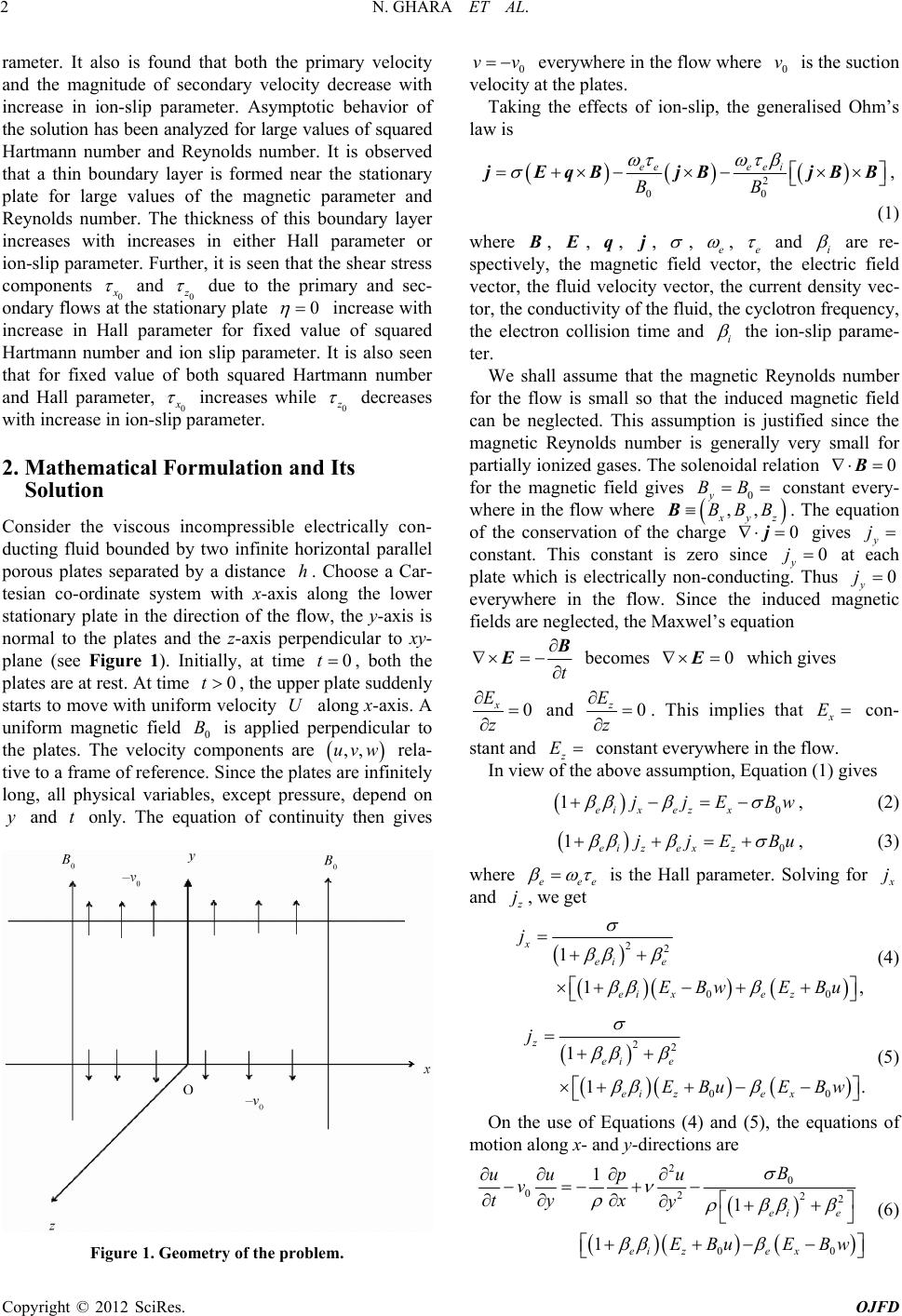 N. GHARA ET AL. 2 rameter. It also is found that both the primary velocity and the magnitude of secondary velocity decrease with increase in ion-slip parameter. Asymptotic behavior of the solution has been analyzed for large values of squared Hartmann number and Reynolds number. It is observed that a thin boundary layer is formed near the stationary plate for large values of the magnetic parameter and Reynolds number. The thickness of this boundary layer increases with increases in either Hall parameter or ion-slip parameter. Further, it is seen that the shear stress components 0 x and 0 z due to the primary and sec- ondary flows at the stationary plate 0 increase with increase in Hall parameter for fixed value of squared Hartmann number and ion slip parameter. It is also seen that for fixed value of both squared Hartmann number and Hall parameter, 0 x increases while 0 z decreases with increase in ion-slip parameter. 2. Mathematical Formulation and Its Solution Consider the viscous incompressible electrically con- ducting fluid bounded by two infinite horizontal parallel porous plates separated by a distance . Choose a Car- tesian co-ordinate system with x-axis along the lower stationary plate in the direction of the flow, the y-axis is normal to the plates and the z-axis perpendicular to xy- plane (see Figure 1). Initially, at time , both the plates are at rest. At time , the upper plate suddenly starts to move with uniform velocity along x-axis. A uniform magnetic field 0 is applied perpendicular to the plates. The velocity components are rela- tive to a frame of reference. Since the plates are infinitely long, all physical variables, except pressure, depend on and only. The equation of continuity then gives h t U 0 uv 0t B ,,w yt Figure 1. Geometry of the problem. 0 vv everywhere in the flow where is the suction velocity at the plates. 0 v Taking the effects of ion-slip, the generalised Ohm’s law is 2 00 eeee i BB jEqBjBjB B, (1) where , B E , , , qj , e , e and i are re- spectively, the magnetic field vector, the electric field vector, the fluid velocity vector, the current density vec- tor, the conductivity of the fluid, the cyclotron frequency, the electron collision time and i the ion-slip parame- ter. We shall assume that the magnetic Reynolds number for the flow is small so that the induced magnetic field can be neglected. This assumption is justified since the magnetic Reynolds number is generally very small for partially ionized gases. The solenoidal relation 0 B for the magnetic field gives constant every- where in the flow where 0y BB ,, x y BBB j z B 0 . The equation of the conservation of the charge gives y j constant. This constant is zero since y at each plate which is electrically non-conducting. Thus 0 0 y j j everywhere in the flow. Since the induced magnetic fields are neglected, the Maxwel’s equation t B E becomes 0 E which gives 0 x E z and 0 z E z . This implies that x E con- stant and z E constant everywhere in the flow. In view of the above assumption, Equation (1) gives 0 1ei xezx jjEB w, (2) 0 1ei zexz jjEB u e , (3) where ee is the Hall parameter. Solving for x j and z j, we get 22 00 1 1, x ei e eixe z j EBwEBu (4) 22 00 1 1. z ei e eize x j EBu EBw (5) On the use of Equations (4) and (5), the equations of motion along x- and y-directions are 2 0 0222 00 1 1 1 ei e eize x B uu pu v ty x y EBu EBw (6) Copyright © 2012 SciRes. OJFD 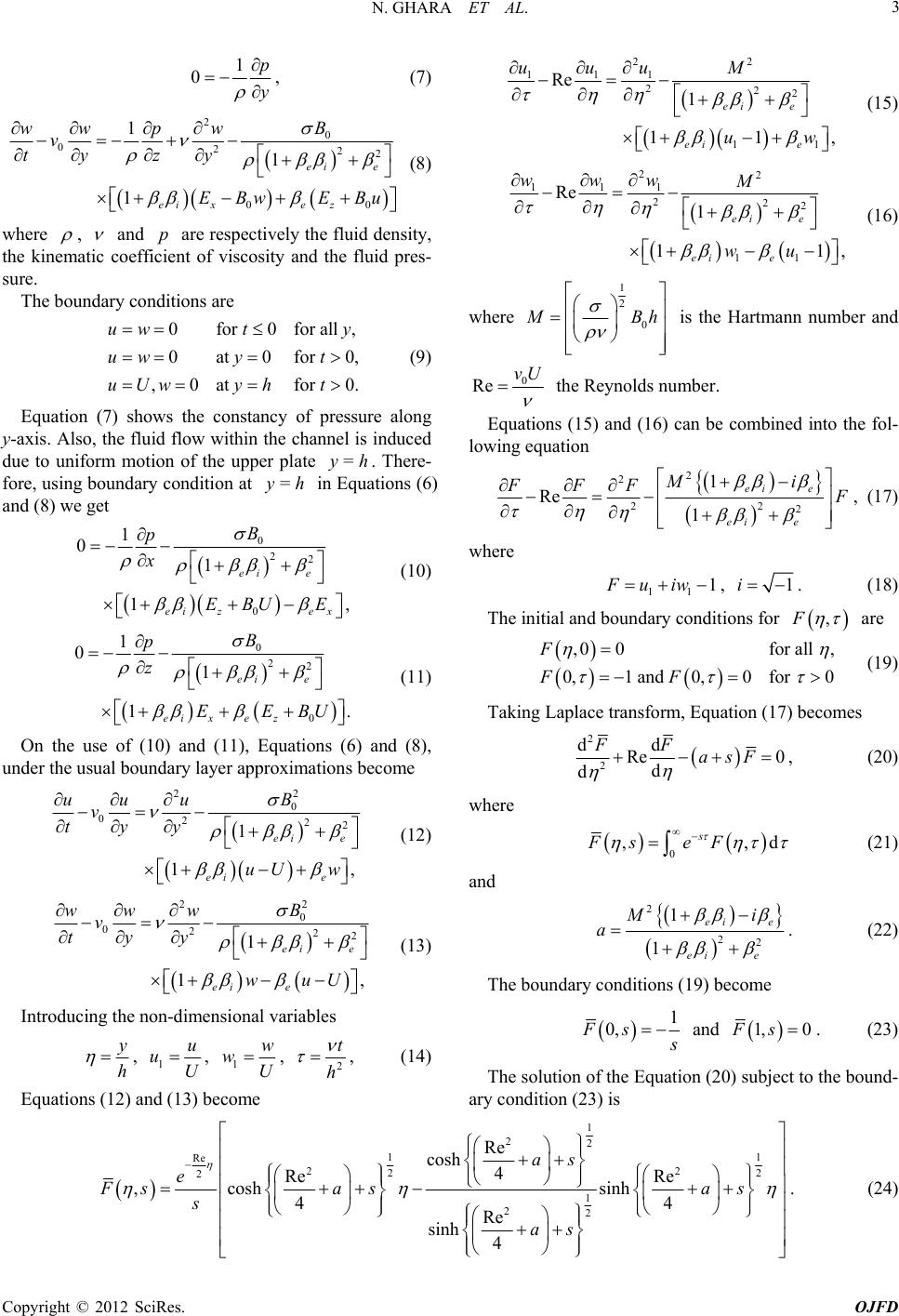 N. GHARA ET AL. Copyright © 2012 SciRes. OJFD 3 1 0p y , (7) EBu 2 0 0222 00 1 1 1 ei e eixe z B wwp w v ty z y EBw (8) where 22 111 222 11 Re 1 11, ei e ei e uuu M uw (15) 22 111 222 11 Re 1 11, ei e ei e wwwM wu (16) , and are respectively the fluid density, the kinematic coefficient of viscosity and the fluid pres sure. The boundary conditions are cy of pressure along y-axis. Also, the fluid flow within the channel is induced due to uniform motion of the upper plate fore, using boundary condition at and (8) we get p - where 1 2 0 M Bh is the Hartmann number and 0 Re vU the Reynolds number. 0for 0for all ,0at for 0. uw ty uUwyh t , 0at 0for 0,uwyt (9) Equation (7) shows the constanEquations (15) and (16) can be combined into the fol- lowing equation =yh in Equat . There- ions (6) =yh 0 22 1 0 1 1, ei e B p x EBU E (10) 2 2 22 2 1 Re 1 ei e ei e Mi FFF F , (17) where 0ei z ex 11 1Fuiw , 1i. (18) The initial and boundary conditions for ,F are 0 22 0 1 0 1 1. ei e ei xe z B p z EEBU On the use of (10) and (11), Equations (6) and (8), under the usual boundary layer approximations become ,00for all , 0,1 and 0,0for 0 F FF (11) (19) Taking Laplace transform, Equation (17) becomes 2 2 dd Re 0 d d FF asF , (20) 2 2 0 0222 1ei e B uu u v ty y 1, ei e uU w where (12) 0 , s Fs eF ,d (21) and 2 22 1 1 ei e ei e M i a . (22) 2 2 0 0222 1 1, ei e ei e B ww w v ty y wuU (13) Introducing the non-dimensional variables The boundary conditions (19) become 1 0,Fs s and 1, 0Fs. (23) y h , 1 u uU , 1 w wU , 2 t h , Equations (12) and (13) become (14) The solution of the Equation (20) subject to the bound- ary condition (23) is 1 22 1 2co R 1 Re 22 2 2 1 22 Re sh 4 e Re ,cosh sinh 44 Re sinh 4 as e Fs asas as s . (24) 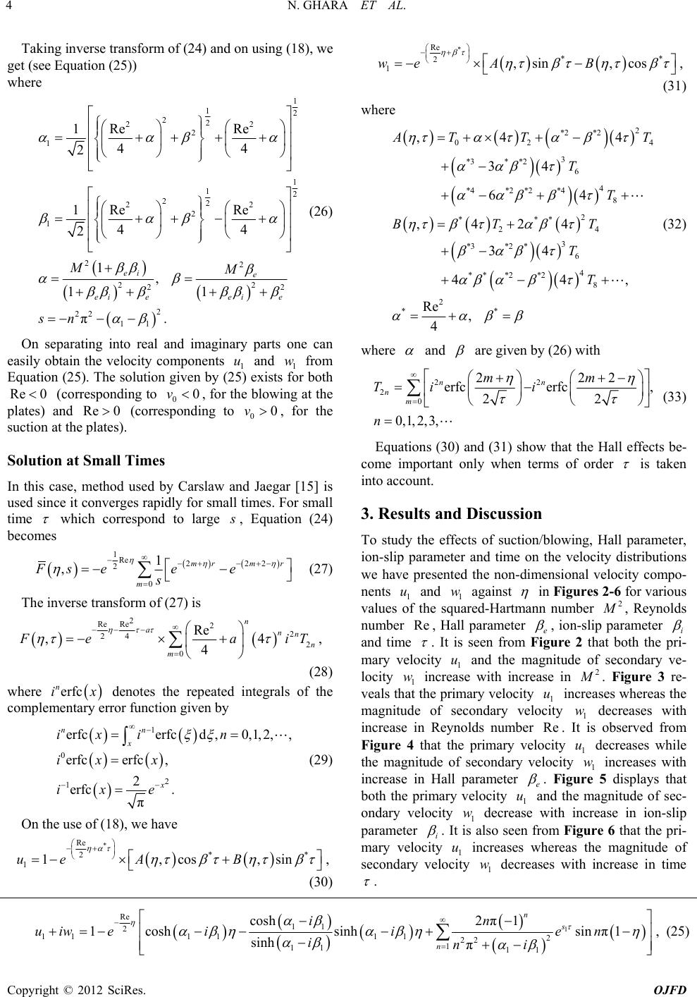 N. GHARA ET AL. 4 Taking inverse transform of (24) and on using (18), we get (see Equation (25)) where 1 12 22 22 2 1 1 12 22 22 1R e 2 22 22 22 2 22 11 1Re Re 44 2 Re 44 2 1, 11 π. ei e ei eei e MM sn (26) On separating into real and imaginary parts one can easily obtain the velocity components and Equation (25). The solution given by (25) exists both (corresponding to 1 1 u1 w for from Re 000v , spond foe blowing at the nd (correing r the Solution at Small Times In or r th to v plates) a suction at the Re 0 plates). 00, fo this case, method used by Carslaw and Jaegar [15] is used since it converges rapidly for small times. F small time which correspond to large s , Equation (24) s become Re 22 21 ,mr r Fs e 1 2 0 m m e e s (27) 7) is The inverse transform of (2 2 Re Re2 2 24 2 0 Re ,4 4 n annn m F eaiT , (28) where n ix erfc lementary err denotes the repeated integrals of the compor function given by 1 0 erfcerfc d x ixi 2 1 ,0,1, 2,, erfcerfc , 2 erfc . π nn x n ixx ix e (29) e use of On th(18), we have * Re * 2 1,cosue AB * 1,sin , (30) * Re ** 2 1,sin ,coswe AB , (31) where 2 *2 *2 02 4 3 *3* *2 6 4 *4*2 *2*4 8 2 *** 24 3 *3*2 * 6 4 * **2*2 8 ** ,4 4 34 64 ,424 34 44, Re , 4 A 2 TT T T T BTT T T where (32) and are given by (26) with 22 2 0 22 erfc erfc, 22 0,1, 2,3, nn nm mm Ti i n 2 (33 Equations (30) and (31) show that the Hall effects be- come important only when terms of order ) is taken into account. 3. Results and Discussion To study the effects of suction/blowing, Hall para ion-slip parameter and time on the velocity distrib we have presented the non-dimensional velocity compo- nents and against meter, utions 1 u1 w in Figures 2-6 for various values the sred-Hartmnn number ofquaa2 M , Reynolds num eber Re , Hall paramter e , ion-slip eter parami and time . It is 1 u se seen frFigure 2both the and the mde ndary om that of seco pri- ve-mary velocity 1 wagnitu locity increa with increase in 2 M . Figure 3 veals tary velocity incwhereas maf ndaryases increase es numed Figure 4ary ases th re- the while h gnitude in at the o R th prim seco ynold at the prim 1 u locity Re velocity r 1 w t 1 u eases decre is observ decre ve ber I with from . e magnitude of secondary velocity 1 w increases with increase in Hall parameter e . Figure 5 displays that both the primary velocity u and the magnitude of sec- ondary veloci 1 ty w1 decrease with increase in ion-slip parameter i . It is also seen from mary velocity u increases whe e Figure 6 s the that the pri- gnitude 1 secondary velocity 1 w decreases with increase in time ra ma of . 1 Re 11 2 11 11112 22 1 11 11 cosh2 π1 1coshsinhsin π1 sinh π n s n in uiweiie n ini , (25) Copyright © 2012 SciRes. OJFD  N. GHARA ET AL. 5 Figure 2. Velocity profiles for M2 when Re = 5, βe = 0.5, βi = 0.5 and τ = 0.02. Figure 3. Velocity profiles for Re when M2 = 5, βe = 0.5, βi = 0.5 and τ = 0.02. For small values of time, we have drawn the velocity components and on using the exact solution given by Equation (25) and the series solution given by Equations (30) and (31) in Figures 7, 8. It is seen that the series solution given by (30) and (31) converge more quickly than the exact solution given by (25) for small time. Hence we conclude that for small time, the nu- merical values of the velocities can be calculated from the Equations (30) and ( an 1 u1 w 31) instead of Equation (25). The non-dimensional shear stresses due to the primary d the secondary velocities at the stationary plate 0 are given by 0 2 22 111 1 11 0 Re π 4 2 2 122 2 2 22 2 sinh2sin2 d1Re d2 cosh2cos2 Re π 1 Re 4 x n n u e n 4 πcossin ,n (34) Copyright © 2012 SciRes. OJFD  N. GHARA ET AL. 6 Figure 4. Velocity profiles for βe when M2 = 5, Re = 5, βi = 0.5 and τ = 0.02. Figure 5. Velocity profiles forβi when M2 = 5, Re = 5, βe = 0.5 and τ = 0.02. 0 2 22 1111 1 11 0 Re π 4 2 2 122 2 2 22 πsin , 4 n 2 sinh2sin2 d dcosh2cos2 Re π 4 Re cos z n n w e n (35) where , , 1 and 1 are given by (26). Numsults he non-dimensional shear stresses erical reof t and 0 z 0 x due to the primary and secondary flows at plate the0 2 are shown graphically in Fig- ures 9-ains 12 agt M for different values of e , i , Re and . Figure ows that the shear st 9 shresses 0 x and 0 z due to thary and the secondary f plate e prim 0 lows at the stationary increase withcrease in in Hall parameter e for fixed value of 2 M , an of , i d . Re 2 It is seen from Figure 10 that for fixed value M , Copyright © 2012 SciRes. OJFD  N. GHARA ET AL. 7 Figure 6. Velocity profiles for time τ wh en M2 = 5, Re = 5, βi = 0.5 and βe = 0.5. Figure 7. Velocity profiles for general solution and small time solution when M2 = 5, Re = 5, βe = 0.5 and βi = 0.5. e , and . Re0 x increases while 0 z decrease parameter with increase in ion-slipi . shows that for fixed value of Figure 11 2 M , 0 x increases while 0 z . Fur- decreases with increase ds number in Reynol Re Copyright © 2012 SciRes. OJFD  N. GHARA ET AL. 8 Figure 8. Velocity profiles for general solution and small time solution when M2 = 5, Re = 5, βe = 0.5 and βi = 0.5. for βe when Re = 5, βi = 0.5 and τ = 0.02. Figure 9. Shear stresses and z0 x0 Copyright © 2012 SciRes. OJFD  N. GHARA ET AL. 9 for βi when Re = 5, βe = 0.5 and τ = 0.02. Figure 10. Shear stresses and zx 0 0 for Re when βe = 0.5, βi = 0.5 and τ = 0.02. Figure 11. Shear stresses and z0 x0 Copyright © 2012 SciRes. OJFD  N. GHARA ET AL. Copyright © 2012 SciRes. OJFD 10 Figure 12. Shear stresses x and z0 0 . ther, it is also found from Figure 12 that both for time τ when βe = 0.5, βi = 0.5 and Re = 5 0 x and 0 z decrease with increase in time for fixe of d value 2 M , i , e and timehear plate Re . s, the sFor small stress at the 0 due to the primary and the secondary flows can be ob- tained as 0 *** 0, 1 0,cos0,sin, 2 x u U eC D *1 2 2 ** 3 4 3 *2 **35 6 ,4Re 24Re 34Re, Y DT Y T Y T (39) with (36) 22 d d2 nn TY 1 0 *** 0, 1 0,sin0,cos, 2 z w U eC D (40) and , (37) where * 11 02 2 *2 *23 4 3 *3* *25 6 ,Re 4Re 4Re 34Re, YY CT T Y T Y T 2121 21 0 22 2 erfcerfc , 22 0,1, 2,3, nn nm mm Yi i n (41) For small time, the numerical values of the shear stress components calculated from Equations (34)-(37) are given in Tables 1 and 2 for different values of (38) e and . It is observed that for small times the shear stresses calculated from the Equations (36) and (37) give better result than that calculated from Equations (34) an(35). d  N. GHARA ET AL. 11 Table 1. Shear stresse M = 1. s due to primary flow for2 = 5, S x (For General solution) x (Solution for small times) e 0.005 0.010 0.015 0.005 0.010 0.015 0.0 5.896093 3.644242 2.6733815.896093 3.6442382.673358 0.5 6.032860 3.765285 2.7827676.032872 3.7653582.782959 1.0 6.290388 3.998794 2.9982426.290404 3.9988862.998493 1.5 6.515985 4.208713 3.1962426.515995 4.2087623.196378 Table 2. Shear stresses due to secondary flow for M2 = 5, S = 1. y (For General Solution) y (Solution for small times) e 0.005 0.010 0.015 0.005 0.010 0.015 0.0 0.000000 0.000000 0.0000000.000000 0.0000000.000000 0.5 0.393570 0.361540 0.3374860.393615 0.3617900.338174 1.0 0.595888 0.555407 0.5247760.595908 0.5555170.525087 1.5 0.660252 0.622620 0.5940050.660258 0.6226500.594089 4. Steady state solution The steady state velocity components are obtained from (25) by letting as (see Equation (42)) Now, we shall discuss the following cases: Case 1): When 21 M and . In this case, Equation (42) gives Re 1 1 Re 2 1cose 11 u , (4) 3 1 Re 2 11 sinwe , (44) re whe 1 2 1 1, ei M 22 11 22 2 1 . 11 ei e e ei eei M (45) It is seen from Equations (43) and (44) that there exists a single-deck boundary layer of thickness of the order 1 1 Re O2 where 1 is given by (45). It i that the thickness of this boundary layer increases with in either Hall parameter s seen increase e or ion-slip pa- rameter i but it decreases withcrease in either Hartmaber in nn num M or Reynoldsber. Case 2): When num Re . ions given by (42) become Re 1, 21 M In this case, the velocity distribut 1 11 1cosue , (46) 1 11 sinwe , (47) where 2 122 2 2 12 22 1 Re 1, Re 1 . Re 1 ei ei e e ei e M M (48) Equations (46) and (47) show the existence of single- deck boundary layer of thickness of order 1 1 O where 1 creases with in is given by (48). The thickness of increase in either Hall parameter this layer e or ion-sliprameter pai as 1 decreases with in either crease in e or i . 5. Single Plate Motion As , the velocity distribution given by (42) be- comes h 1 2 11 1co S ue s , 9) (4 1 2 S 11 sinwe , (50) where 1 12 22 22 2 1 1 12 22 22 2 1 2 2 00 2 1, 44 2 1 44 2 , , SS SS vB Uz SM UU (51) and , are given by (26). It is clear from above Equations (49) and (50) that the flow exhibits a boundary layer behavior with boundary layer thickness of order of 1 1 O2 S . Since 1 increases with increase in either or S2 M it means that increase in either suction pa- Re 112 111111 11 cosh 1sinhcosh sinh i uiwii e i (42) Copyright © 2012 SciRes. OJFD  N. GHARA ET AL. 12 rameter or magnetic parameter S 2 M causes thinning of the ary layer. Further, fod and boundr fixeS2 M and 0 z , 1 decrwith increase in eithrameter eases er Hall pae or ion-parameter slip i . Hence, nclude that t boundary layer thickness near the we co plate he 0 increases with increase in either e or i . The solutions given by (49) and (50) are also valid for the blowing (<0S) at the plate. In thsence of ion e ab-slip (0 i ), the above Equa- tions (49)d (50) be ancome 2 11cosue S , (52) 2 1sin S we , (53) where 1 2 2 22 22 22 4 411 2 e e e i 22 1 2 2 2 2, 1 22 2 2 22 1M SM 1 2 2 2 M 2. 1SM 11 2 41 41 eM e e e e SM S (54) Equations (52) and (53) coincide with Equatons (36) and (37) of Gupta [16] when 0 i (abse ce of on th tte flow n two iite ho boun layer imas have been studied. It is founat th mary vcity decreases while th nda velo increases with increase in e n dary d th ion- e un- rizon- ap- e pri- Hall slip). 6. Conclusion Co ste tal prox seco param mbined effects of Hall current and ion-slip ady MHD Couebetweenfin parallel porous plates under the tion elo ry ter 1 u city e magnitude of 1 w e . It is magni in also tude ion-slip found that bot of secondary velcity decrease parameter h the primary ve- locity and with incr t ea he se o i . obse at a th form e fouof magnetic r It is ed near the stationa ete rved ry th plat in r la boun rge da val ry layer is es param2 M and Reynolds. The thickne these boary layers increases with increases in either Hall parameter or ion-slip parameter. Further, it is seen that the shear stresses number Ress ofund 0 x due to the primary and secondary flows at plate the stationary 0 increase with in- crease in Hall paramter ee for fixed value of 2 M . It is also seen thfixeat for d value of 2 M , 0 x while increases 0 z decrease with increase in ion-slip pater rame i . REFE nd P ineers and Appli h o p /TPS.1979.4317226 RE S.-I. e NCES d [1] [2] K. R. Crammer for Eng New York, 1973 Heat Trans Vol. 7, N doi:10.1109 a . ai, “Magnetofluid Dynamics Physicists,” McGraw-Hill, V. M. Soundalgekar, N. V. Vighnesam and H. S. Takhar, “Hall and Ion-Slip Effects in MHD Couette Flow wit fer,” IEEE Transactions on Plasma Science, . 3, 1978, p. 178-182. [3] H. A. Attia, “Unsteady Couette Flow with Heat Transfer Considering Ion-Slip,” Turkish Journal of Physics, Vol. 29, 2005, pp. 379-388. [4] H. A. Attia, “Ueady Couette Flow with H Tnst c F “Time 47. “Anal rcul Attia, “Transient Hart 75. /Phy e Slip,” and Ion Slip CEC cripta atfer luid . Var Hydro between Parallel Porous Journal of Technical P . 131-1 ttia,ytil Solution for Flow of y i Hall eering Communications, . mann ering the Ion,” . 470-4 sica.R .066 rans Journal a Dust Effects,” ), Vol. 194 of a Viscoelasti Consider ying ca ar Pipe with . 1287-1296 Slip egular ing the Ion magn Plate hys ( Flow with Physica S a00470 of the Korean Physical Society, Vol. 47, No. 5, 2005, pp. 809-817 A. Attia, Fluid Ion Slip,” 2006, pp . A Fluid in a C Chemical Engin No. 10, 2007, pp A. fer Consid 2002, pp doi:10.1238 [5] [7] H. ty H. etic Flow of Dus- s Considering the ics, Vol. 47, No. 3, [6] H. A Heat Trans- , Vol. 66, [8] M. A. Seddeek, “The Effects of Hall and Ion-Slip Cur- rents on Magneto-Micropolar Fluid and Heat Transfer over a Non-Isothermal Stretching Sheet with Suction and Blowing,” Proceedings of the Royal Soceity: London A, Vol. 457, 2001, pp. 3039-3050. doi:10.1098/rspa.2001.0847 [9] P.am, “Th C. R Free Convectiv e EffecHall and Ion-Slip Cur e Heat Generating Flow in a al of Energy ol. 6. doi:10.1002/er.444 ts of n rents on Rotating ch, V 0190502 Fluid,” International Jour 19, No. 5, 1995, pp. 371-37 Resear in a MHD Channel with Hall and Ion Applie Research . 18216 [10] M. LMittal and A. N. Bhat, “Forced Convective Heat Tran . sfer rents,” pp. 251-264 Slip Cur- d Scientific doi:10.1007/BF004 , Vol. 35, No. 4, 1979, N. Jana and ouette Flow tating S,” Acta Meccanica . 301-3/BF01177152 [11] R. N. ystem 06. Datta, “C doi:10.1007 and Heat Transfer , Vol. 26, No. 1-4, in a Ro 1977, pp [12] Kanch na, “ Hal Flowy Layer Approximations,” nal of the Physical Sciences, Vol. 7, 2001, pp. 74-86. [13] H. A. Attia, “Ion Slip Effect on Unsteady Couette Flow A. K. tte and R. u N. Ja nder Boundar l Effect on Unsteady Coue Jour Copyright © 2012 SciRes. OJFD  N. GHARA ET AL. Copyright © 2012 SciRes. OJFD 13 with Heat Transfer under Exponential Decaying Pressure Gradient,” Tamkang Journal of Science and Engineering, Vol. 12, No. 2, 2009, pp. 209-214. [14] B.K. Jha and C. A. Apere, “Combined Effect of Hall and Ion-Slip Currents on Unsteady MHD Couette Flows in a Rotating System,” Journal of the Physical Society of Ja- pan, Vol. 79, No. 10, 2010, pp. 104401-104401-9. doi:10.1143/JPSJ.79.104401 [15] H. S. Carslaw and J. C. Jaegnduction of Heat in S er, “Co olids,” Oxford University Press, Oxford, 1959. dromagnetic Flow Past a Porous Flat Effects,” Acta Mechanica, Vol. 22, No. [16] A. S. Gupta, “Hy Plate with Hall 3-4, 1975, pp. 281-287. doi:10.1007/BF01170681 |