Wireless Sensor Network, 2010, 2, 358-364
doi:10.4236/wsn.2010.24047 Published Online May 2010 (http://www.SciRP.org/journal/wsn)
Accurate Angle-of-Arrival Measurement Using
Particle Swarm Optimization
Minghui Li, Kwok Shun Ho, Gordon Hayward
Centre for Ultrasonic Engineering, University of Strathclyde, Glasgow, UK
Received December 4, 2009; revised February 22, 2010; accepted March 19, 2010
Abstract
As one of the major methods for location positioning, angle-of-arrival (AOA) estimation is a significant
technology in radar, sonar, radio astronomy, and mobile communications. AOA measurements can be ex-
ploited to locate mobile units, enhance communication efficiency and network capacity, and support loca-
tion-aided routing, dynamic network management, and many location-based services. In this paper, we pro-
pose an algorithm for AOA estimation in colored noise fields and harsh application scenarios. By modeling
the unknown noise covariance as a linear combination of known weighting matrices, a maximum likelihood
(ML) criterion is established, and a particle swarm optimization (PSO) paradigm is designed to optimize the
cost function. Simulation results demonstrate that the paired estimator PSO-ML significantly outperforms
other popular techniques and produces superior AOA estimates.
Keywords: Array Signal Processing, Angle-of-Arrival (AOA) Estimation, Location Positioning, Particle Swarm
Optimization, Smart Antennas
1. Introduction
Estimation of the incident signals’ directions, or angle-of-
arrival (AOA) estimation, is a fundamental problem in
numerous applications such as radar, sonar, radio as-
tronomy, and mobile communications. AOA measure-
ments can locate mobile units, and thus support and en-
hance location-aided routing, dynamic network planning
and management, and different types of location-based
services and applications [1], furthermore, it can improve
communication efficiency and network capacity when
integrated with adaptive array technology.
In general, location estimates of mobile units are de-
rived from two types of measurements: AOA and range.
The widely used range estimation models include re-
ceived signal strength (RSS), time of arrival (TOA) and
time difference of arrival (TDOA), where cooperation
and synchronization between the transmitter and receiver
are required [1]. On the contrary, the AOA model can
locate targets in a non-cooperative, stealthy and passive
manner, which is highly desirable in military and sur-
veillance applications. The benefits of AOA measure-
ments for location estimation have been widely investi-
gated, and many AOA-alone [2-4] and hybrid systems
[5-8] ha ve been proposed.
A chief goal of wireless communication research has
long been to enhance the network capacity, data rate and
communication performance. In comparison with solu-
tions of increasing spectrum usage, smart antenna tech-
nology provides a more practical and cost-efficient solu-
tion. The benefits of using smart antennas are that the
sender can focus the transmission energy towards the
desired user while minimizing the effect of interference,
and the receiver can form a directed beam towards the
sender while simultaneously placing nulls in the direc-
tions of the other transmitters. This spatial filtering capa-
bility leads to increased user capacity, reduced power
consumption, lower bit error rates (BER), and larger
range coverage [9,10]. A key component that aids the
array to be ‘smart’ and adaptive to the environment is
AOA estimation of the desired signals and co-channel
interferers. To fully exploit the AOA capability in mobile
communications, various Medium Access Control (MAC)
protoc ols have been de ve l oped [11-13].
In recent years, AOA estimation has received consid-
erable attention from radar and communication commu-
nities, and several high resolution algorithms have been
proposed based on the white Gaussian noise model, such
as multiple signal classification (MUSIC) [14], maxi-
mum likelihood (ML) [15], and others [16,17]. However,
in many circumstances, the emitters reside in a “radio

M. H. LI ET AL.359
L
hostile” environment and the noise fields tend to be cor-
related along the array due to the dominant ambient noise
[18]. Furthermore, the systems are often forced to work
under unfavorable conditions involving low signal-to-
noise ratio (SNR), highly correlated signals, and small
array with few elements due to the cost, energy and size
constraints. The standard AOA techniques become in-
competent in such scenarios.
In this paper, we propose an algorithm for accurate
AOA measurement in colored noise fields and harsh ap-
plication scenarios. By modeling the unknown noise co-
variance as a linear combination of known weighting
matrices, a maximum likelihood criterion is derived with
respect to AOA and unknown noise parameters. ML cri-
teria may yield superior statistical performance, but the
cost function is multimodal, nonlinear and high-dimen-
sional. To tackle it efficiently, we propose to use the par-
ticle swarm optimization (PSO) paradigm as a robust and
fast global search tool. PSO is a recent additio n to evolu-
tionary algorithms first introduced by Eberhart and Ken-
nedy [19]. Most of the applications demonstrated that
PSO could give competitive or even better results in a
much faster and cheaper way, compared to other heuris-
tic methods such as genetic algorithms (GA) [20].
The PSO is designed to combine the problem-inde-
pendent kernel and problem-specific features, which
make the algorithm highly flexible while being specific
and effective in the current application. Via extensive
numerical studies, we demonstrate that the proposed al-
gorithm yields superior performance over other popular
methods, especially in unfavorable scenarios involving
low SNR, highly correlated signals, short data samples,
and small arrays.
The paper has been organized as follows. Section 2
describes mathematical models of the signal and noise,
and derives the ML criterion function. In Section 3,
PSO-ML and the strategies for parameter selection are
presented. Simulation results are given in Section 4, and
Section 5 concludes the paper.
2. Data Model and Problem Formulation
We consider an array of M elements arranged in an arbi-
trary geometry and N narrowband far-field sources at
unknown locations. The complex M-vector of array out-
puts is modeled by the standard equation
()( )()(),1,2,...,ttttyAθsn (1)
where is the source AOA vector, and
the kth column of the complex
1
[, ,]
T
N
 θ
M
N matrix


A

is the so called steering vector

k

a for the angle k

.
The ith element

ik
a


models the gain and phase ad-
justments of the kth signal at the ith element. Further-
more, the complex N-vector


ts is composed of the
emitter signals, and


tn models the additive noise.
The vectors of signals and noise are assumed to be sta-
tionary, temporally white, zero-mean complex Gaussian
random processes with second-order moments given by










0
0
s
s
s



H
T
H
T
Et
Et
Et
Et




ts
ts
s






Pss
ss
nn
nn
Q
(2)
where ts

is the Kronecker delta,

H
 denotes com-
plex conjugate transpose, denotes transpose, and

T


E stands for expectation. Assuming that the noise
and signals are independent, the data covariance matrix
is given by
 


H
t
H
Et

Ryy APAQ (3)
Moreover, it is assumed that the number of sources is
known or has been estimated using techniques, e.g., in
[21]. The problem addressed herein is the estimation of
(and if necessary, along with the parameters in P and
Q) from a batch of L measurements , …,
θ

1y


Ly.
Under the assumption of additive Gaussian noise and
Gaussian distributed signals, the normalized (with L)
negative log-likelihood fun ction of the data v ectors takes
the form (ignoring the parameter independent terms) [22]


1ˆ
,,

gtr

PQ RRloI R (4)
where


tr  stands for trace, log  denotes the natu-
ral logarithm of the determinant, and is the covari-
ance matrix of the measured data
ˆ
R
1
1
ˆ()
L
t
t
L
 Ry ()
H
ty
1
(5)
In the follows, we focus on the ML criterion derived
using parameterization of the noise covariance. Because
this assumption applies no constraints to the signals, it is
applicable to both cooperative and non-cooperative sce-
narios.
Based on a Fourier series expansion of the spatial
noise power density function, the noise covariance Q is
assumed to be modeled by the following linear parame-
terization [18]:

J
j
j

j
 QηΣ (6)
where 1,..., T
J
 




η is a vector of unknown noise

M. H. LI ET AL. 360
Fourier coefficients,
j
Σ is a known function of the ar-
ray geometry given by
(1)/2
/2
odd
even
j
j
j
j
j






Σ
ΣΣ
 (7)
where
 
 
cos
sin
H
l
H
l
ld
ld














Σaa
Σaa


(8)
0, 1,2,l. It is assumed that j is known or has been
estimated [18,21]. Similar descriptive models depicting
the noise covariance as a linear combination of known
weighting matrices are widely accepted in the literature
[18,21,23,24].
Following the derivation in [25], P can be solved in
terms of and Q,

Aθ

η
 
1
ˆHHHH




PAAARA AAAA1 (9)
paradigm, which mimics animal social behaviors such as
flocking of birds and the methods by which they find
roosting places or food sources [19]. PSO starts with the
initialization of a population of individuals in the search
space and works on the social behavior of the particles in
the swarm. Each particle is assigned a position in the
problem space, which represents a candidate solution to
the problem under consideration. Each of these particle
positions is scored to obtain a scalar cost, named fitness,
based on how well it solves the problem. These particles
then fly through the problem space subject to both de-
terministic and stochastic update rules to new positions,
which are subsequently scored. Each particle adaptively
updates its velocity and position according to its own
flying experience and its companions’ flying experience,
aiming at a better position for itself. As the particles tra-
verse the search space, each particle remember its own
personal best position that it has ever visited, and it also
knows the best position found by any particle in the
swarm. On successive iterations, each particle takes the
path of a damped oscillatory movement towards its per-
sonal best and the global best positions. With the oscilla-
tion and stochastic adjustment, particles explore regions
throughout the problem space and eventually settle down
near a good solution.
where
1/2
1/2 1/2
ˆ.




AQ A
RQ RQ
(10)
By substituting (9) back to (3) and (4), the ML crite-
rion function can be finally reduced to


1,loglogI ηQGRGHH

trR (11)
where

1
H
H



GAAA A
HIG
(12)
The ML estimates of and are obtained by
minimizing (11). Based on the data model, the Cramer-
Rao bound (CRB) for AOA estim ation can be derived [18],
η
In Equation (13),


Re  represents the real part,
denotes element-wise product, and

 
1N
 









aa
D

J
(14)
As illustrated in Figure 1, the algorithm starts by ini-
tializing a population of particles in the “normalized”
search space with random positions x and random ve-
locities v, which are constrained between zero and one in
each dimension. The position vector of the ith particle
takes the form11 ,...,, ,...,
iN








x

, where 0,
n



1
j


, 1,...,nN

, 1,...,jJ

, , . A parti-
cle position vector is converted to a candidate solution
vector in the problem space through a mapping. The
score of the mapped vector evaluated by the likelihood
function
1N1J


η
1,I (11) is regarded as the fitness of the
corresponding particle.
The ith particle’s velocity is updated according to (15)


1112 2 kkkkkk kk
ii iig
cc 
 vvrpxrpx

k
i
(15)
where pi is the best previous position of the ith particle,
pg is the best position found by any particle in the swarm,
1, 2,k

, indicates the iterations,

is a parameter
called the inertia weight, and are positive con-
stants referred to as cognitive and social parameters re-
spectively, and are independent random vectors.
1
c2 c
1
r2 r
3. PSO-ML AOA Estimation and Parameter
Selection
Particle swarm optimization is a stochastic optimization




1
11 11
1
CRB Re
2
TT
HH HH
L

 




θPA RAPDRDPA RDPA RD
(13)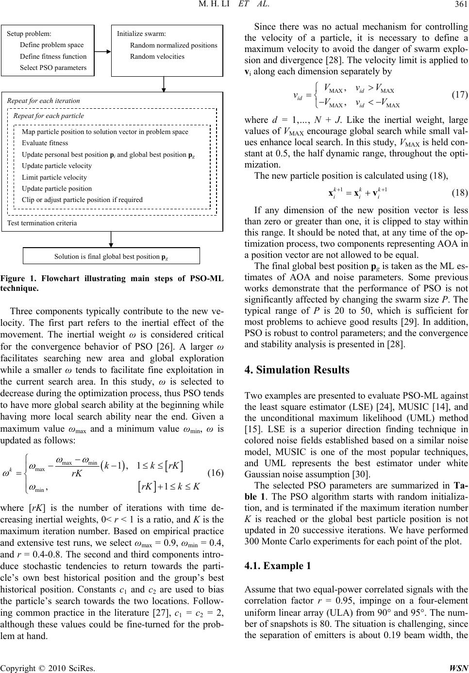

M. H. LI ET AL. 361
Repeat for each iteration
Repeat for each particle
Map particle position to solution vector in problem space
Evaluate fitness
Update pers onal bes t position p
i
and global best position p
g
Update particle velocity
Limit par t icle velo ci ty
Update particle position
Clip or adj ust par t icle posi tio n if required
Test terminatio n cr it er ia
Setup problem:
Define problem space
Define fitness function
Select PSO parameters
Initializ e swar m:
Random normalized positions
Random veloc i ti e s
Solution is final glo b al best po sit io n p
g
Figure 1. Flowchart illustrating main steps of PSO-ML
technique.
Three components typically contribute to the new ve-
locity. The first part refers to the inertial effect of the
movement. The inertial weight ω is considered critical
for the convergence behavior of PSO [26]. A larger ω
facilitates searching new area and global exploration
while a smaller ω tends to facilitate fine exploitation in
the current search area. In this study, ω is selected to
decrease during the optimization process, thus PSO tends
to have more global search ability at the beginning while
having more local search ability near the end. Given a
maximum value ωma x and a minimum value ωmin, ω is
updated as follows:
 

max min
max
min
1, 1
,
kkkrK
rK
rKk K








 
1
1
(16)
where [rK] is the number of iterations with time de-
creasing inertial weights, 0< r < 1 is a ratio, and K is the
maximum iteration number. Based on empirical practice
and extensive test runs, we select ωmax = 0.9, ωmin = 0.4,
and r = 0.4-0.8. The second and third components intro-
duce stochastic tendencies to return towards the parti-
cle’s own best historical position and the group’s best
historical position. Constants c1 and c2 are used to bias
the particle’s search towards the two locations. Follow-
ing common practice in the literature [27], c1 = c2 = 2,
although these values could be fine-turned for the prob-
lem at hand.
Since there was no actual mechanism for controlling
the velocity of a particle, it is necessary to define a
maximum velocity to avoid the danger of swarm explo-
sion and divergence [28]. The velocity limit is applied to
vi along each dimension separately by
MAX MAX
MAX MAX
,
,
id
id
id
VvV
vVvV



 (17)
where d = 1,…, N + J. Like the inertial weight, large
values of VMAX encourage global search while small val-
ues enhance local search. In this study, VMAX is held con-
stant at 0.5, the half dynamic range, throughout the opti-
mization.
The new particle position is calculated using (18),
1kkk
iii


xxv (18)
If any dimension of the new position vector is less
than zero or greater than one, it is clipped to stay within
this range. It should be noted that, at any time of the op-
timization process, two components representing AOA in
a position vector are not allowed to be equal.
The final global best position pg is taken as the ML es-
timates of AOA and noise parameters. Some previous
works demonstrate that the performance of PSO is not
significantly affected by changing the swarm size P. The
typical range of P is 20 to 50, which is sufficient for
most problems to achieve good results [29]. In addition,
PSO is r obu s t to contr o l p arameters; and the convergence
and stability analysis is presented in [28].
4. Simulation Results
Two examples are presented to evaluate PSO-ML against
the least square estimator (LSE) [24], MUSIC [14], and
the unconditional maximum likelihood (UML) method
[15]. LSE is a superior direction finding technique in
colored noise fields established based on a similar noise
model, MUSIC is one of the most popular techniques,
and UML represents the best estimator under white
Gaussian noise assumption [ 3 0].
The selected PSO parameters are summarized in Ta-
ble 1. The PSO algorithm starts with random initializa-
tion, and is terminated if the maximum iteration number
K is reached or the global best particle position is not
updated in 20 successive iterations. We have performed
300 Monte Carlo experiments for each point of the plot.
4.1. Example 1
Assume that two equal-power correlated signals with the
correlation factor r = 0.95, impinge on a four-element
uniform linear array (ULA) from 90 and 95. The num-
ber of snapshots is 80. The situation is challenging, since
the separation of emitters is about 0.19 beam width, the

M. H. LI ET AL. 362
Table 1. Selected PSO parameters.
Parameter Value
c1 2.0
c2 2.0
P 20
K 200
M
AX
V 0.5
max

0.9
min

0.4
r 0.5
conventional resolution limit. The noise covariance is
modeled as a linear combination of known matrices (6),
J = 3, and


1,1/4,1/9η. Similar noise models are
used in the literature [29]. Figure 2 depicts the combined
AOA estimation root-mean-squared errors (RMSE) ob-
tained using PSO-ML, LSE, MUSIC and UML as a
function of SNR, and compares them with the corre-
sponding CRB (13) (theoretically best performance).
Figure 3 shows the resolution probabilities for the same
methods. Two sources are considered to be resolved in
an experiment if both estimation errors are less than the
half of their angular separation.
As can be seen from Figures 2 and 3, PSO-ML yields
significantly superior performance over LSE, MUSIC
and UML as a whole, by demonstrating lower estimation
RMSE and higher resolution probabilities. PSO-ML
produces excellent AOA estimates with RMSE ap-
proaching and asymptotically attaining the theoretic
510 15 20 2530
10-1
100
101
102
SNR (dB)
RM SE (d egre e)
PSO-ML
LS E
UML
MUSIC
CRB
Figure 2. AOA estimation RMSE of PSO-ML, LSE, MUSIC
and UML versus SNR. Dashdot line represents theoretic
CRB. Two correlated sources impinge on four-element
ULA at 90 and 95, r = 0.95. Number of snapshots is 80.
-5 05 10 15 20 25 30
0
0.2
0.4
0.6
0.8
1
S NR (d B)
Res ol ution P roba bi l i ty
PSO-ML
LS E
UML
MUSIC
Figure 3. Resolution probabilities of PSO-ML, LSE, MU-
SIC and UML versus SNR. Two correlated sources impinge
on four-element ULA at 90 and 95, r = 0.95. Number of
snapshots is 80.
lower bound. On the other hand, as a standard high- res-
olution method, MUSIC fails almost in the whole SNR
range. Although UML is an optimal technique in white
Gaussian noise, it completely fails when SNR is lower
than 15 dB and only produces acceptable estimates in
high SNR region. It is worth noting that the advantages
of PSO-ML over the other methods are more prominent
when SNR is low, and the benefits can be extended to
other unfavora ble conditions .
4.2. Example 2
In the second example, we consider an 8-element ULA.
Two emitters are present at 80 and 83 with a sepa-
ration of 0.23 beamwidth, r = 0.9. The number of
snapshots is 30. In the noise model (6), J = 5 and


1,0.75,0.5,0.25,0.1η. Figure 4 illustrates the RMSE
values obtained from PSO-ML, LSE, MUSIC and UML.
The resolution probabilities for the same methods are
shown in Figure 5.
As expected, PSO-ML significantly outperforms LSE,
MUSIC and UML and produces more accurate estimates
by showing lower RMSE and higher resolution prob-
abilities. We select a different scenario in this example,
although the source separation in terms of array beam-
width is similar, the data sample is much shorter and
there is more freedom in the noise model as compared
with Example 1. As shown in Figures 2-5, the benefits
of PSO-ML over LSE with colored noise model and
UML and MUSIC under white Gaussian noise assump-
tion appear to be more prominent in unfavorable scenar-
ios involving low SNR, short data samples, closely
spaced and highly corr elated sour ces, an d unkno wn noise
environment.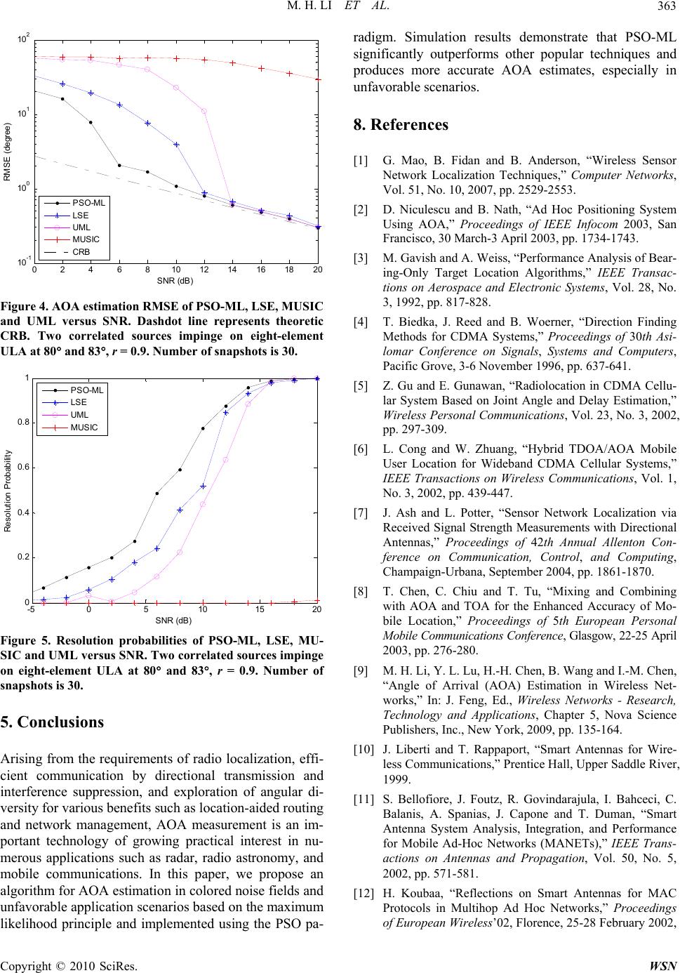

M. H. LI ET AL.363
0 24681012 14 16 1820
10
-1
10
0
10
1
10
2
S NR (dB)
RMSE (degree)
PSO-ML
LS E
UML
MUSIC
CRB
Figure 4. AOA estimation RMSE of PSO-ML, LSE, MUSIC
and UML versus SNR. Dashdot line represents theoretic
CRB. Two correlated sources impinge on eight-element
ULA at 80 and 83, r = 0.9. Number of snapshots is 30.
-5 05 10 15 20
0
0.2
0.4
0.6
0.8
1
SNR
(
dB
)
Resolution Probabilit y
PSO-ML
LS E
UM L
MUSIC
Figure 5. Resolution probabilities of PSO-ML, LSE, MU-
SIC and UML versus SNR. Two correlated sources impinge
on eight-element ULA at 80 and 83, r = 0.9. Number of
snapshots is 30.
5. Conclusions
Arising from the requirements of radio localization, effi-
cient communication by directional transmission and
interference suppression, and exploration of angular di-
versity for various benefits such as location-aided routing
and network management, AOA measurement is an im-
portant technology of growing practical interest in nu-
merous applications such as radar, radio astronomy, and
mobile communications. In this paper, we propose an
algorithm for AOA estimation in colored noise field s and
unfavorable application scenarios based on the maximum
likelihood principle and implemented using the PSO pa-
radigm. Simulation results demonstrate that PSO-ML
significantly outperforms other popular techniques and
produces more accurate AOA estimates, especially in
unfavorabl e scenarios.
8. References
[1] G. Mao, B. Fidan and B. Anderson, “Wireless Sensor
Network Localization Techniques,” Computer Networks,
Vol. 51, No. 10, 2007, pp. 2529-2553.
[2] D. Niculescu and B. Nath, “Ad Hoc Positioning System
Using AOA,” Proceedings of IEEE Infocom 2003, San
Francisco, 30 March-3 April 2003, pp. 1734-1743.
[3] M. Gavish and A. Weiss, “Performance Analysis of Bear-
ing-Only Target Location Algorithms,” IEEE Transac-
tions on Aerospace and Electronic Systems, Vol. 28, No.
3, 1992, pp. 817-828.
[4] T. Biedka, J. Reed and B. Woerner, “Direction Finding
Methods for CDMA Systems,” Proceedings of 30th Asi-
lomar Conference on Signals, Systems and Computers,
Pacific Grove, 3-6 November 1996, pp. 637-641.
[5] Z. Gu and E. Gunawan, “Radiolocation in CDMA Cellu-
lar System Based on Joint Angle and Delay Estimation,”
Wireless Personal Communications, Vol. 23, No. 3, 2002,
pp. 297-309.
[6] L. Cong and W. Zhuang, “Hybrid TDOA/AOA Mobile
User Location for Wideband CDMA Cellular Systems,”
IEEE Transactions on Wireless Communications, Vol. 1,
No. 3, 2002, pp. 439-447.
[7] J. Ash and L. Potter, “Sensor Network Localization via
Received Signal Strength Measurements with Directional
Antennas,” Proceedings of 42th Annual Allenton Con-
ference on Communication, Control, and Computing,
Champaign-Urbana, September 2004, pp. 1861-1870.
[8] T. Chen, C. Chiu and T. Tu, “Mixing and Combining
with AOA and TOA for the Enhanced Accuracy of Mo-
bile Location,” Proceedings of 5th European Personal
Mobile Communications Conference, Glasgo w, 22-25 Ap ril
2003, pp. 276-280.
[9] M. H. Li, Y. L. Lu, H.-H. Chen, B. Wang and I.-M. Chen,
“Angle of Arrival (AOA) Estimation in Wireless Net-
works,” In: J. Feng, Ed., Wireless Networks - Research,
Technology and Applications, Chapter 5, Nova Science
Publishers, Inc., New York, 2009, pp. 135-164.
[10] J. Liberti and T. Rappaport, “Smart Antennas for Wire-
less Communications,” Prentice Hall, Upper Saddle River,
1999.
[11] S. Bellofiore, J. Foutz, R. Govindarajula, I. Bahceci, C.
Balanis, A. Spanias, J. Capone and T. Duman, “Smart
Antenna System Analysis, Integration, and Performance
for Mobile Ad-Hoc Networks (MANETs),” IEEE Trans-
actions on Antennas and Propagation, Vol. 50, No. 5,
2002, pp. 571-581.
[12] H. Koubaa, “Reflections on Smart Antennas for MAC
Protocols in Multihop Ad Hoc Networks,” Proceedings
of European Wireless’02, Florence, 25-28 February 2002,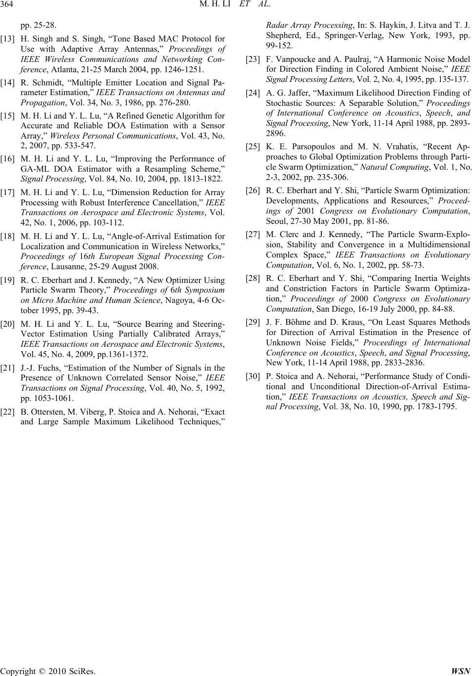

M. H. LI ET AL. 364
pp. 25-28.
[13] H. Singh and S. Singh, “Tone Based MAC Protocol for
Use with Adaptive Array Antennas,” Proceedings of
IEEE Wireless Communications and Networking Con-
ference, Atlanta, 21-25 March 2004, pp. 1246-1251.
[14] R. Schmidt, “Multiple Emitter Location and Signal Pa-
rameter Estimation,” IEEE Transactions on Antennas and
Propagation, Vol. 34, No. 3, 1986, pp. 276-280.
[15] M. H. Li and Y. L. Lu, “A Refined Genetic Algorithm for
Accurate and Reliable DOA Estimation with a Sensor
Array,” Wireless Personal Communications, Vol. 43, No.
2, 2007, pp. 533-547.
[16] M. H. Li and Y. L. Lu, “Improving the Performance of
GA-ML DOA Estimator with a Resampling Scheme,”
Signal Processing, Vol. 84, No. 10, 2004, pp. 1813-1822.
[17] M. H. Li and Y. L. Lu, “Dimension Reduction for Array
Processing with Robust Interference Cancellation,” IEEE
Transactions on Aerospace and Electronic Systems, Vol.
42, No. 1, 2006, pp. 103-112.
[18] M. H. Li and Y. L. Lu, “Angle-of-Arrival Estimation for
Localization and Communication in Wireless Networks,”
Proceedings of 16th European Signal Processing Con-
ference, Lausanne, 25-29 August 2008.
[19] R. C. Eberhart and J. Kennedy, “A New Optimizer Using
Particle Swarm Theory,” Proceedings of 6th Symposium
on Micro Machine and Human Science, Nagoya, 4-6 Oc-
tober 1995, pp. 39-43.
[20] M. H. Li and Y. L. Lu, “Source Bearing and Steering-
Vector Estimation Using Partially Calibrated Arrays,”
IEEE Transactions on Aerospace and Electronic Systems,
Vol. 45, No. 4, 2009, pp.1361-1372.
[21] J.-J. Fuchs, “Estimation of the Number of Signals in the
Presence of Unknown Correlated Sensor Noise,” IEEE
Transactions on Signal Processing, Vol. 40, No. 5, 1992,
pp. 1053-1061.
[22] B. Ottersten, M. Viberg, P. Stoica and A. Nehorai , “Exact
and Large Sample Maximum Likelihood Techniques,”
Radar Array Processing, In: S. Haykin, J. Litva and T. J.
Shepherd, Ed., Springer-Verlag, New York, 1993, pp.
99-152.
[23] F. Vanpoucke and A. Paulraj, “A Harmonic Noise Model
for Direction Finding in Colored Ambient Noise,” IEEE
Signal Processing Letters, Vol. 2, No. 4, 1995, pp. 135-137.
[24] A. G. Jaffer, “Maximum Likelihood Direction Finding of
Stochastic Sources: A Separable Solution,” Proceedings
of International Conference on Acoustics, Speech, and
Signal Processing, New York, 11-14 April 1 988, p p. 2893-
2896.
[25] K. E. Parsopoulos and M. N. Vrahatis, “Recent Ap-
proaches to Global Optimization Problems through Parti-
cle Swarm Optimization,” Natural Computing, Vol. 1, No.
2-3, 2002, pp. 235-306.
[26] R. C. Eberhart and Y. Shi, “Particle Swarm Optimization:
Developments, Applications and Resources,” Proceed-
ings of 2001 Congress on Evolutionary Computation,
Seoul, 27-30 May 2001, pp. 81-86.
[27] M. Clerc and J. Kennedy, “The Particle Swarm-Explo-
sion, Stability and Convergence in a Multidimensional
Complex Space,” IEEE Transactions on Evolutionary
Computation, Vol. 6, No. 1, 2002, pp. 58-73.
[28] R. C. Eberhart and Y. Shi, “Comparing Inertia Weights
and Constriction Factors in Particle Swarm Optimiza-
tion,” Proceedings of 2000 Congress on Evolutionary
Computation, San Diego, 16-19 July 2000, pp. 84-88.
[29] J. F. Böhme and D. Kraus, “On Least Squares Methods
for Direction of Arrival Estimation in the Presence of
Unknown Noise Fields,” Proceedings of International
Conference on Acoustics, Speech, and Signal Processing,
New York, 11-14 April 1988, pp. 2833-2836.
[30] P. Stoica and A. Nehorai, “Performance Study of Condi-
tional and Unconditional Direction-of-Arrival Estima-
tion,” IEEE Transactions on Acoustics, Speech and Sig-
nal Processing, Vol. 38, No. 10, 1990, pp. 1783-1795.