Applied Mathematics
Vol.5 No.1(2014), Article ID:41934,22 pages DOI:10.4236/am.2014.51018
Pseudo DNA Sequence Generation of Non-Coding Distributions Using Variant Maps on Cellular Automata
1School of Software, Yunnan University, Kunming, China
2School of Life Sciences, Yunnan University, Kunming, China
Email: *conjugatesys@gmail.com
Received September 19, 2013; revised October 19, 2013; accepted October 26, 2013
ABSTRACT
In a recent decade, many DNA sequencing projects are developed on cells, plants and animals over the world into huge DNA databases. Researchers notice that mammalian genomes encoding thousands of large noncoding RNAs (lncRNAs), interact with chromatin regulatory complexes, and are thought to play a role in localizing these complexes to target loci across the genome. It is a challenge target using higher dimensional tools to organize various complex interactive properties as visual maps. In this paper, a Pseudo DNA Variant MapPDVM is proposed following Cellular Automata to represent multiple maps that use four Meta symbols as well as DNA or RNA representations. The system architecture of key components and the core mechanism on the PDVM are described. Key modules, equations and their I/O parameters are discussed. Applying the PDVM, two sets of real DNA sequences from both the sample human (noncoding DNA) and corn (coding DNA) genomes are collected in comparison with two sets of pseudo DNA sequences generated by a stream cipher HC-256 under different modes to show their intrinsic properties in higher levels of similar relationships among relevant DNA sequences on 2D maps. Sample 2D maps are listed and their characteristics are illustrated under a controllable environment. Various distributions can be observed on both noncoding and coding conditions from their symmetric properties on 2D maps.
Keywords:Large Noncoding; DNA Analysis; Stream Cipher; HC-256; Binary to DNA; Pseudo DNA Sequence; Visual Distribution; Variant Map
1. Introduction
Finding a proper generation mechanism for specific functional DNA sequences is a challenge task in the modern bioinformatics. DNA sequences are composed of four meta symbols on {A,C,T,G}. From an algebraic viewpoint, it is feasible to transfer any 0 - 1 sequence under Cellular Automata following a 2 bits transforming table to generate pseudo DNA sequences. Considering different configurations, there is 24 = 4! possible rules in transformation. Considering generations of 0 - 1 sequences, pseudo random number generation mechanism [1,2] takes the central position in modern cryptography [3-6]. Associated with advanced development of bioinformatics, advanced DNA sequencing and analyzing techniques [7-24] have significantly progressed over the past decade.
1.1. Large Non-Coding DNA & RNA
In DNA analysis, visualization methods play a key role in the Human Genome Project (HGP) [8]. After HGP completed successfully, a public research consortium, the Encyclopedia of DNA Elements (ENCODE) was launched by the National Human Genome Research Institute (NHGRI) in 2003 to find all functional elements in the human genome.
In 2012, ENCODE released a coordinated set of 37 papers published in key Journals of Nature, Science, Genome Biology and Genome Research. These publications show that approximately 20% of non-coding DNA in the human genome is functional while an additional 60% is transcribed with no known function [13]. Much of this functional non-coding DNA is involved in the regulation of the expression of coding genes [14].
Furthermore the expression of each coding gene is controlled by multiple regulatory sites located both near and distant from the gene. These results demonstrate that gene regulation is far more complex than previously believed [15]. Mammalian genomes encode thousands of large non-coding RNAs (lncRNAs), many of which regulate gene expression, interact with chromatin regulatory complexes, and are thought to play a role in localizing these complexes to target loci across the genome [17]. Associated with different international projects, larger numbers of Genome Databases are established and mass Genome-wide gene expression measurements are developed over the world.
1.2. DNA Analysis
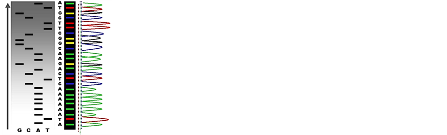
DNA analysis plays a key role in modern genomic application [8]. The HGP is heavily relevant to advanced DNA sequencing and analysis techniques. DNA sequences are composed of four Meta symbols on {A,T,G,C} as basic structure. Classical DNA double helix structure makes the first level of pair construction of DNA sequences with A:T and G:C complementary structures on the first level of symmetric relationships. A typical DNA sequencing result is shown in Figure 1(a). Four Meta symbols could be separated as four projective sequences.
In ENCODE, recent Genomic analysis results are indicated that encoded sequences have only 20 percent in human genomes and around 80 percent genomes look like useless sequences. Under further assumptions, it seems that additional symmetric properties are required to satisfy the second, third and higher levels of structural constructions to explore complex interactive properties [8-18].
In current situation, it is necessary for advanced researchers to shift focus in computational cell biology from directly sequencing data to making higher-level interpretation and exploring efficient content-based retrieval mechanism for genomes.
1.3. DNA Cryptography
DNA cryptography makes joined research in the field of DNA computing and cryptography. Different results are published such as simulating DNA evolution [3], DNA pseudorandom number generator [7,19,20,23], DNA cryptography [4,21,22] and so on.
In typical results of DNA cryptography on encryption, different coding schemes could be randomly selected. E.g. the algorithm in paper [21] applies an encoding formula to express the plaintext on DNA sequence: {00 → C, 01 → T, 10 → A, 11 → G}; however in paper [22], the same author uses the coding formula {00 → A, 01 → T, 10 → C, 11 → G} for the plaintext on DNA sequence. In encryption environment, all 24 possible encoding methods could be equally used in different applications.
1.4. Stream Cipher HC-256
Stream ciphers are an important class of encryption algorithms. A stream cipher is a symmetric cipher which operates with a time-varying transformation on individual plaintext digits. HC-256 is a stream cipher designed to provide bulk encryption in software at high speeds while permitting strong confidence in security. A 128-bit variant was submitted in 2004 as an eSTREAM cipher candidate; it has been selected as one of the four final contestants in the software profile [6] in 2008 as the most advanced scheme in modern network environment.
1.5. Variant Construction and DNA
Variant construction is a new structure on Cellular Automata composed of logic, measurement and visualization models to analyze 0 - 1 sequences under variant conditions. The further details of this construction can be checked on variant logic [25,26], 2D maps [27,28], variant pseudo-random number generator [29-31], DNA maps [32,33] and dynamic properties on variant phase spaces [28]. Since the variant construction uses another set of four Meta symbols  to describe relevant systems, a typical correspondence shown in Figure 1(b) may provides a natural mapping between DNA and variant data sequences.
Since DNA sequences are played an essential role to explore different symmetric properties based on analysis approaches, in this paper, measurement and visual models are proposed systematically to use a fixed segment structure to measure four Meta symbols distributions in their spectrum construction. Under this construction, refined symmetric features can be identified from various polarized distributions and further symmetric properties are visualized.
1.6. Target of This Paper
This paper establishes a Pseudo DNA Variant Map (PDVM) following Cellular Automata. The PDVMis a unified framework to analyze complex DNA interactions for both artificial and natural DNA sequences. This paper provides an extending version on [33] that proposed an initial framework VMS to support some simulation properties for mode = 1 cases only. The PDVM has designed to use variant logic schemes on Cellular Automata [25-33] applying multiple maps on four Meta symbols as DNA or RNA representations. System architecture of key components and core mechanism on the PDVM are described. Key modules, equations and their I/O parameters are discussed. Applying the PDVM, two sets of real DNA sequences from both human (non-coding DNA) and corn (coding DNA) genomes are collected in comparison with two sets of pseudo DNA sequences generated by HC-256 on mode = {1,2} to show their intrinsic properties in higher levels of similar relationships among DNA sequences on 2D maps. Further descriptions and discussions are systematically provided respectively.
2. System Architecture
In this section, system architecture and their core components are discussed with the use of diagrams. The refined definitions and equations of this system are described in the next section—Pseudo DNA Variant Map.
Specific symbols for groups are listed as follows:
 An integer indicates the t-th DNA sequence selected,
 An integer indicates a relationship distance among elements in a binary sequence,
 An integer indicates the mode of elements in a sequence,
  , mode = 0 for a DNA sequence, mode = {1,2} for a binary sequence
 An integer indicates the number of elements in the t-th DNA sequence,
 An input data vector with
  elements,
 An integer indicates the number of elements in a segment,
V A symbol is selected from four DNA symbols ,
, 
 An integer indicates the control parameter for mapping,
 A unified DNA vector with
  elements,
 Four sets of probability measurements with
 Four paired values,
 (a)
(a)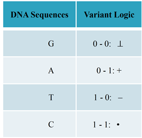 (b)
(b)
Figure 1. Modern DNA sequencing & correspondences on Variant Logic. (a) A sample DNA sequencing and its four projection sequences; (b) Four Meta DNA Symbols and linkages to Variant Logic.
 Four 2D maps,
 Four 0 - 1 vectors with
  elements,
 Four histograms for relevant probability measurements,
 Four normalized histograms for relevant probability measurements,
∀t All DNA sequences are selected, 
2.1. Architecture
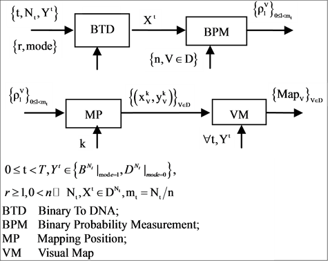
The four components of a PDVM are the Binary To DNA (BTD), the Binary Probability Measurement (BPM), the Mapping Position (MP), and the Visual Map (VM) as shown in Figure 2.
The architecture is shown in Figure 2(a) with the key modules of the four core components being shown in Figures 2(b)-(e) respectively.
In the first part of the system, the t-th sequence  on either {0,1} or {A,G,T,C} are input data to get into the BTD module. The main function of the BTM is to output a unified sequence
  either to transfer a 0 - 1 sequence or to keep a pseudo DNA sequence as a pseudo or pure DNA sequence under a set of controlled parameters. Under different mode condition, various lengths can be identified between input 0 - 1 sequence and output pseudo DNA sequence.
 (a)
(a)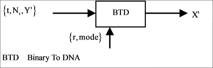 (b)
(b)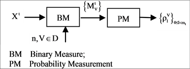 (c)
(c)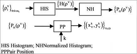 (d)
(d)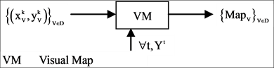 (e)
(e)
Figure 2. Pseudo DNA Variant Map PDVM and key components (a) Architecture of PDVM composed of four components: BTD, BPM, MP and VM; (b) BTD Binary to DNA module is itself: BTD; (c) BPM Binary Probability Measurement module is composed of two components: BM and MP; (d) MP Mapping Position module is composed of three components: HIS, NH and PP; (e) VM module is itself: VM.
Using this unified DNA sequence, four vectors of probability measurements are created from the t-th selected DNA sequence with  elements as an input. Multiple segments are partitioned by a fixed number of n elements for each segment; at least
  segments can be identified by the BPM component. Next component uses the four vectors of probability measurements and a given k value as input data, a pair of position values are created for each Meta symbol. Four pairs of values are generated by the MP component. Then, in order to process multiple selected DNA sequences, all selected sequences are processed by the VM component and each sequence may provide a set of pair values to generate relevant variant maps to indicate their distribution properties respectively.
With eight parameters in an input group, there are three sets of parameters in the intermediate group and one set of parameters in the output group.
The three groups of parameters are listed as follows.
Group:
 ,
,  ,
,  ,
,
 ,
,  ,
,
 ,
,  ,
, 
Group:
 ,
,  ,
,

Group:

2.2. BTD Binary to DNA
The BTD component shown in Figure 2(b) is composed of one module: BTD itself. Five parameters are shown as input signals and one unified vector is generated by the BTD component as the output group.
Group:
 ,
,  ,
, 
 ,
, 
Group:

If mode = 2 condition, double number of 0 - 1 elements are required to generate a given length pseudo DNA sequence than mode = 1 condition. The BTD component uses an input vector on either binary or DNA format as input, under a set of input parameters to process transformation. The output of the BTD component is composed of a unified vector of DNA format in a given set of conditions.
2.3. BPM Binary Probability Measurement
The BPM component shown in Figure 2(c) is composed of two modules: BM Binary Measure and PM Probability Measurement. Three parameters are listed as input signals; four vectors of binary measures are outputted from the BM component as an intermediate group and four sets of probability measurements are outputted as an output group.
Group:
 ,
,  ,
, 
Group:

Group:

The BPM component transforms a selected DNA sequence to generate four 0 - 1 vectors by BM module for the input DNA sequence. Then four probability vectors are generated by the PM module as the output of the BPM under a fixed length of segment condition.
2.4. MP Mapping Position
The MP component shown in Figure 2(d) is composed of three modules: HIS Histogram, NH Normalized Histogram and PP Pair Position. Two parameters are listed as input signals; four histograms and four normalized histograms are generated from the HIS component and the NH component as intermediate groups respectively. Four paired values are generated by the PP component as the output group.
Input Group:
 ,
, 
Group:

Group:

The MP component uses probability measurements as input, under a given k condition to generate each relevant histogram and its normalized distribution. The output of the MP component is composed of four paired values controlled in a given condition
2.5. VM Visual Map
The VM component shown in Figure 2(e) is composed of one module: VM Visual Map. Three parameters are input signals. Collected all selected DNA sequences, four 2D maps are generated by the VM component as the output result.
Group:
 ,
,
 ,
,

Output Group:

The VM component processes all selected DNA sequences as input to generate paired values for each sequence. The output of the VM component is composed of four 2D maps to show the final visual distribution for the system.
3. Pseudo DNA Variant Map PDVM
In this section, definitions and equations are provided to describe the PDVM. In addition to the initial preparation, seven core modules are involved in the BTD, BM, PM, HIS, NH, PP and VM components respectively.
3.1. Initial Preparation
Let  an input parameter make all pairs of elements with r distance in a binary sequence to be a pseudo DNA vector,
  a controlled parameter indicate various pairs of operations performed if
 . Denote
  a binary base and
  a DNA base respectively.
3.2. BTD Module
Let  an input sequence with N elements,
  ,
, . This input vector could be expressed as follows.
 (1)
(1)
Let X denote a DNA sequence with N elements, D denote a symbol set with four elements i.e. . This type of a DNA sequence can be described by a four valued vector as follows:
 (2)
(2)
From this input and associated parameters, following operations are performed.
If mode = 0, for all I,  , the output vector is equal to the input vector.
 (3)
(3)
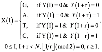
If mode = 1, for all pairs of I and  elements of Y, Y(I),
  , the I-th output element
  can be determined by the corresponding conditions shown in Figure 1(b) as follows.
 (4)
(4)
Under this condition, a 0 - 1 sequence with N elements can generate a pseudo DNA sequence with the same elements.
If mode = 2, only half pairs of I  and
and  elements of Y, Y(I),
  , the I-th output element
  can be determined by the corresponding conditions shown in Figure 1(b) as follows.
 (5)
(5)
Under this condition, a 0 - 1 sequence with N element can generate a pseudo DNA sequence with  elements.
In both conditions,  will be a unified vector with four values as the output of the BTD shown in Figure 2(b).
e.g. Let a binary sequence 
 , three pseudo DNA sequences
  under two mode conditions can be represented as follows.
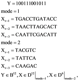
Selecting a certain  value and a fixed mode, a relevant pseudo DNA sequence can be generated from an input binary sequence.
Normal rules of DNA cryptography [21,22] take only r = 1 and mode = 2 conditions for transformations. For mode = 1 situations, normal rules cannot be covered.
From a Cellular Automata viewpoint, this type of transformation plays a key role in the PDVM. This is a significantly distinguishable condition to check whether generated pseudo DNA sequences with/without non-coding properties.
3.3. BM Module
For a given I-th element, four projective operators can be defined and denoted as .
.
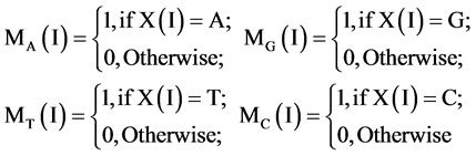 (6)
(6)
Applying the four operators to all elements, the DNA sequence X can be reorganized into the four binary sequences of 0 - 1 values. i.e.
 (7)
(7)
e.g. Let a DNA sequence 
 , its four binary sequences can be represented as follows:
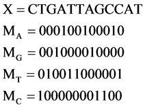
It is interesting to notice that the basic relationship between a DNA sequence X and its four  sequences are exactly same as in a modern DNA sequencing procedure to separate a selected DNA sequence into the four Meta symbol sequences shown in Figure 1(a). This correspondence could be the key feature to apply the proposed scheme naturally in simulating complex behaviors for any DNA sequence.
The projection  provides the essential operation in the BM component as the first module shown in Figure 2(c).
3.4. PM Module
For this set of the four binary sequences, it is convenient to partition them into m segments and each segment contained a fixed number of n elements.
For the l-th segment, let , the I-th position will be
 , four probability measurements
  can be defined.
 (8)
(8)
Under this construction, four sets of probability measurements established.
 (9)
(9)
The probability operator  generates four probability measurement vectors in the PM component as the second module shown in Figure 2(c). After the BM and PM processes, the whole procedure of the BPM component is complete in Figure 2(c).
3.5. HIS Module
Since the BPM generates four sets of probability measurement, it is necessary to perform further operations in the MP component shown in Figure 2(d) as follows.
In the HIS component as the first module in Figure 2(d), each probability sequence  can be calculated from n positions, at most n + 1 distinguished values identified in a vector. Under this organization, a histogram distribution can be established.
Let  be a histogram operator, for each position, it satisfies following relation,
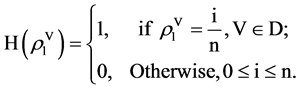 (10)
(10)
Collecting all possible values, a histogram distribution can be established,
 (11)
(11)
The histogram  is the output of the HIS module. Four histograms are generated after HIS process. Further normalized process will be performed in the NH component as the second module in Figure 2(d).
3.6. NH Module
Under this construction, a normalized histogram can be defined as
 (12)
(12)
After the NH component processed, its output provides the PP component for further operations as the third module in Figure 2(d).
3.7. PP Module
Relevant probability vectors have (n + 1) distinguished values; four sets of normalized vectors can be organized as a linear order as follows,
 (13)
(13)
Under this condition, four linear sets of probability vectors are established,
 (14)
(14)
For four vectors, their components can be normalized respectively,
 (15)
(15)
Four sets of probability vectors are composed of a complete partition on their measurements.
Using this set of measurements, two mapping functions can be established to calculate a pair of values to map analyzed DNA sequence into a 2D map as follows.
Let  and
and  or
or  be a pair of values defined by following equations,
 (16)
(16)
In the PP component, four paired values are generated and each pair indicates a specific position on a 2D map for the selected DNA sequence. The core operations of three key components: BTD, BPM and MP for a selected sequence are performed in Figures 2(b)-(d).
3.8. VM Module
Since only one point of a 2D map is determined for a selected DNA sequence, it is essential to apply relativelarger number of DNA sequences as inputs to generate visible distributions. This type of operations will be performed in the VM component shown in Figure 2(e).
In a general condition, the VM component processes a selected data set  composed of T sequences, the t-th sequence with
  elements can be expressed by


Each sequence can be processed to apply the same procedures of the BTD, BPM and MP components. Since for each segment, its length n will be fixed for all selected sequences, it is essential to make number of segments be  in convention to match each sequence. Under this expression, the last module VM collects all T pairs of positions on relevant 2D visual maps as follows,
 (17)
(17)
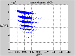
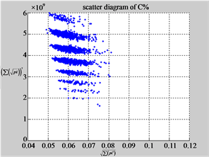
A sample 2D map of VM is shown in Figure 3. This provides an assistant illustration for this type of visual maps on a case of multiple sequences.
Under this construction, a total number of T DNA sequences are transformed as T visual points on four 2D visual maps that would be help analyzers to explore their intrinsic symmetry properties among four binary sequences.
4. Sample Results on 2D Maps
Two types of data sets are selected for comparison. The first type of data sets is real DNA data sequences collected from both human and plan genomes to illustrate their differences on 2D maps. The second type of data set is collected from the Stream Cipher HC-256 to generate a pseudo random binary sequence under a certain condition.
4.1. DNA Data Resources
It is important to use some real DNA sequences to illustrate various test results of the PDVM. Two sets of DNA sequences are selected and relevant resource features are described as follows.
The first data set originally comes from the human genome assembly version 37 and was taken from the reference sequences of 13 anonymous volunteers from Buffalo, New York. Hi-C technology used to analyze chromatin interaction role in genome. From a genomic analysis viewpoint, this set of data may contain more complex secondary or higher level structures. A special structure nearly the GRCh37 DNA sequence has been identified to explore their spatial characteristics. After positive and negative sequencing, each data file contain 2700 DNA sequences and each sequence has around 500 elements stored in one file right.
The second DNA data set are selected from some plant gene database for comparison. One set of DNA sequences of Corn genomes are stored in file 201 - 500 that contains 2700 DNA sequences and each sequence has around 200 - 600 elements. It may be ordinary single sequences without complex secondary structures.
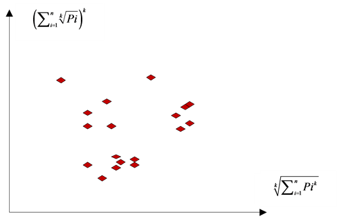
Figure 3. A sample 2D map of VM on multiple sequences.
4.2. Pseudo DNA Data Resources
The Stream Cipher HC-256 has being used to generate a binary sequence on a total length of  (mode = 1) and
  (mode = 2) bits in the file hc256 that has been partitioned as 2700 subsequences and each sub-sequence in 500/1000 bits respectively.
Using the PDVM in various parameters, six sets of pseudo DNA sequences are generated and their 2D maps are illustrated, analyzed and compared in following subsections.
4.3. Sample Results
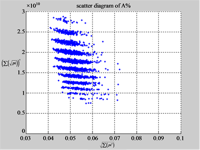
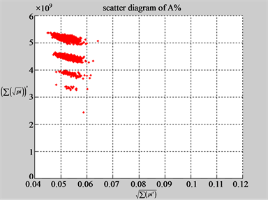
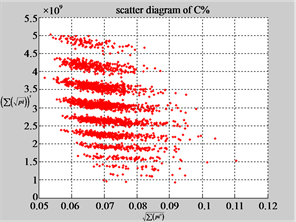
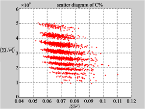
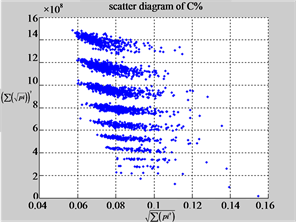
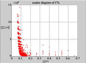
Using the two files of DNA sequences and two pseudo binary sequences in three parameters, relevant 2D maps are listed in Figures 4-7 under different conditions to illustrate their spatial distributions using the PDVM in a controllable environment.
In Figure 4, four groups of sixteen 2D maps are shown in the range of 


 for comparison; (a1 - a4) four
  maps for the file Right; (b1 - b4) four
  maps for the file 201 - 500; (c1 - c4) four
  maps for the file hc256, mode = 1; (d1 - d4) four
 maps for the file hc256, mode = 2 respectively.
In Figure 5, two groups of eight 2D maps for the files right and 201 - 500 are selected in the range of 
 ,
,
 ; (a) group (a1 - a4) four
  maps for file right; (b) group (b1 - b4) four
  maps for the file 201 - 500.
In Figure 6, six groups of twenty four 2D maps for the file hc256 are compared in the range of 


 (a) (c) (e) groups for mode = 1 (a1 - a4) four
  maps r = 1; (c1 - c4) four
  maps r = 2; (e1 - e4) four
  maps r = 3; (b) (d) (f) groups for mode = 2 (b1 - b4) four
  maps r = 1; (d1 - d4) four
  maps r = 2; (f1 - f4) four
  maps r = 3.
In Figure 7, six groups of twenty four 2D maps for three files right, 201 - 500 and hc256 are compared in the range of 

 ; (a) the file right n = 15, mode = 0; (b) the file hc256 n = 12, mode = 1, r = 1; (c) the file hc256 n = 12, mode = 1, r = 3; (d) the file hc256 n = 12, mode = 2, r = 1; (e) the file hc256 n = 12, mode = 2, r = 3; (f) the file 201 - 500, n = 15, mode = 0; (a1 - f1)
  maps; (a2 - f2)
 maps; (a3 - f3)
  maps; (a4 - f4)
  maps.
maps.
4.4. Result Analysis of 2D Maps
Four groups of 2D maps contain different Information, it is necessary to make a brief discussion on their important issues as follows.
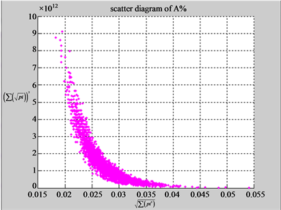
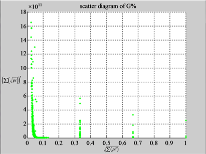
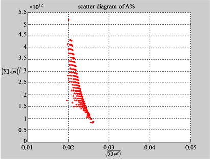
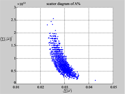
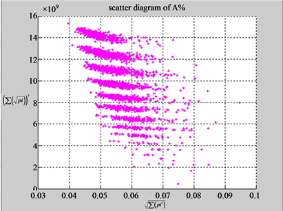
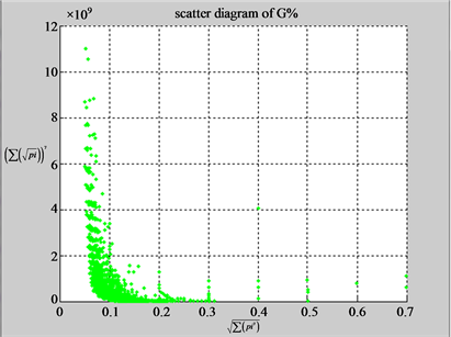
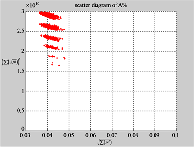
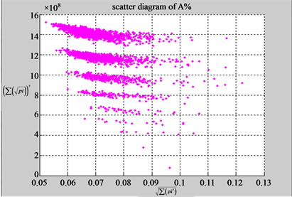
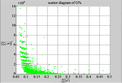
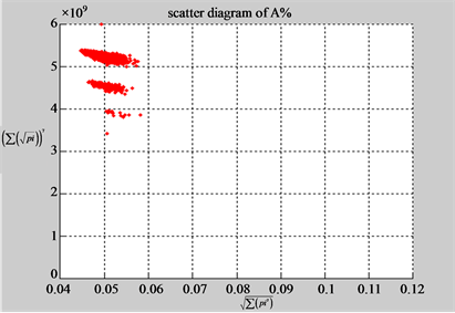
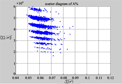
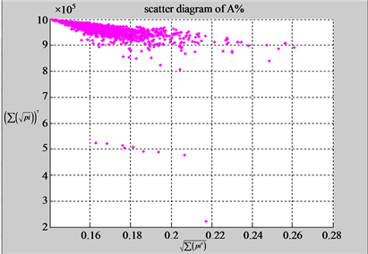
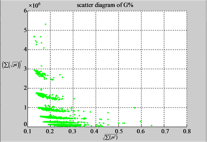
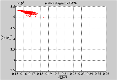
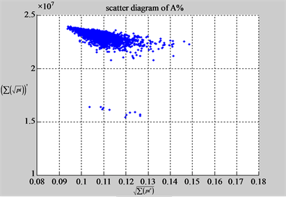
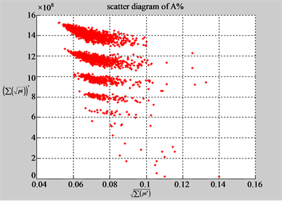
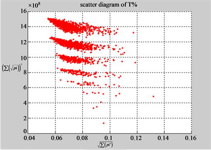
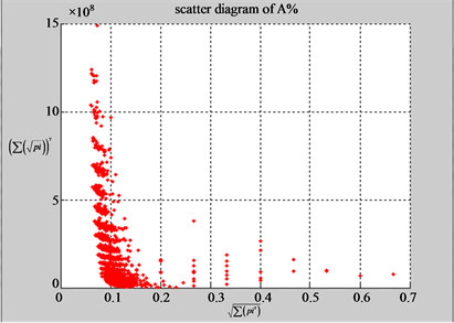
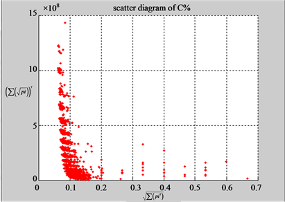
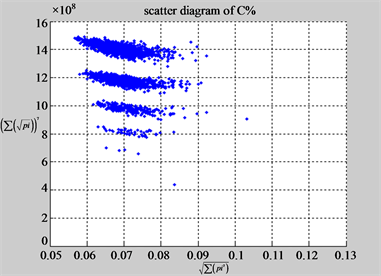
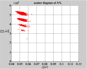
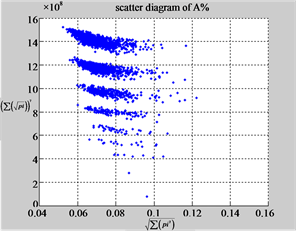
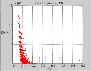
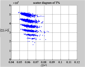
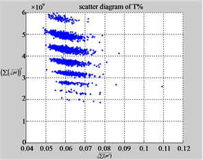
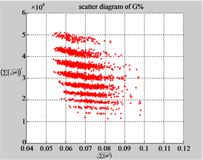
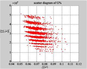
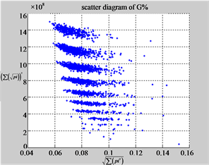
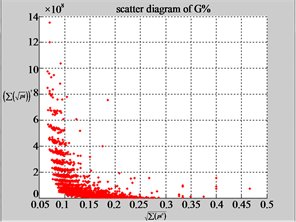
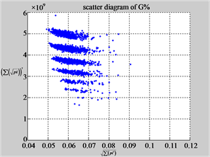
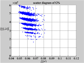
The first group of results shown in Figure 4 presents four sets of sixteen 2D maps from three data files: right, 201 - 500 and hc256 (mode = {1,2}) undertaken various lengths of basic segment from 3 - 50 to illustrate their variations respectively. Four 2D maps of each group in Figure 4 (a1 - a4) show significant trace on their visual distributions; the numbers of main visible clusters identified are decreased when the length of segment has being increased e.g. (a3 - a4). However, lesser length of segment does not provide refined visual distinctions with larger region in fuzzy areas e.g. (a1 - a2). From a structural viewpoint, middle ranged numbers of length provide better clustering results e.g. (a2 - a3) for further analysis targets. To check another four 2D maps of Figure 4 (b1 - b4) for the file 201 - 500, significantly different visual distributions can be observed than (a1 - a4); the numbers of main visible clusters identified are decreased when the length of segment has being increased less significantly e.g. (b1 - b4). However lesser length of segment does not provide refined visual distinctions with wider regions in fuzzy areas e.g. (b1 - b2). In general, middle ranged numbers of length still provide better clustering effects e.g. (b3 - b4) for further analysis purpose. Eight 2D maps of Figure 4 (c - d) (c1 - c4) for the file hc256 r = 1, mode = 1, and (d1 - d4) for the file hc256 r = 1, mode = 2, similar visual distributions can be observed than (a1 - a4) and significantly differences are observed than (b1 - b4); the numbers of main visible clusters identified are decreased when the length of segment has being increased less significantly e.g. (c3 - c4)/(d3 - d4). However lesser length of segment does provide refined visual distinctions with regions in fuzzy areas e.g. (c1)/(d1). In general, middle ranged numbers of length still provide better clustering effects e.g. (c2 - c3)/(d2 - d3) for further analysis purpose. From their distributions, groups (a) and (c - d) have shared much stronger similar properties than Group (b).
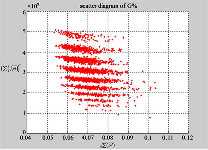
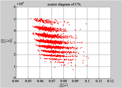
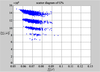
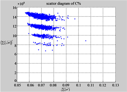
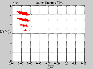
Using a set of selected parameters, two groups of eight 2D maps are compared in Figure 5 for two files: right and 201 - 500 to explore higher levels of symmetric properties for secondary or higher levels of structures
 n = 3: (a1) (b1)
 n = 3: (c1) (d1)
 n = 10: (a2) (b2)
 n = 3: (c2) (d1)
 n = 15: (a3) (b3)
 n = 15: (c3) (d1)
 n = 50: (a4) (b4)
 n = 50: (c4) (d1)
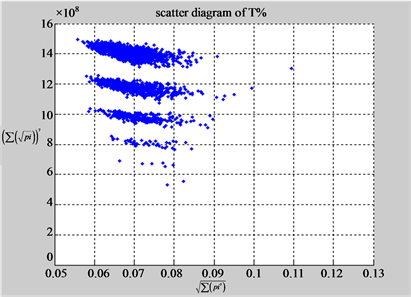
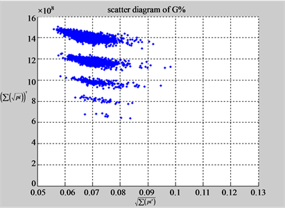
Figure 4. Four groups of sixteen 2D maps in the range of n = 3 - 50, k = 7, N  200 - 600, T = 2700; (a1 - a4) MapA for the file right; (b1 - b4) MapG for the file 201 - 500; (c1 - c4) MapA for the file hc256 mode = 1, r = 1, (d1 - d4) MapA for the filehc256 mode = 2, r = 3.
 (a1) MapA (a2) MapT
 (b1) MapA (b2) MapT
 (a3) MapG (a4) MapC
 (b3) MapG (b4) MapC
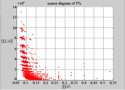
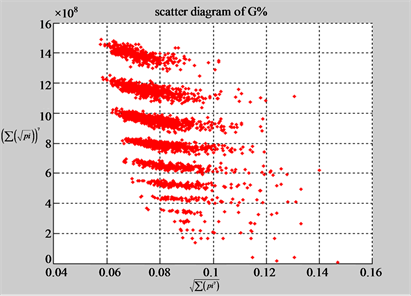
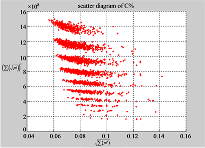
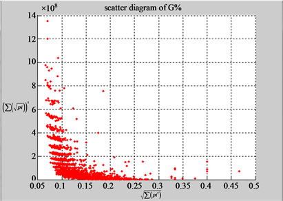
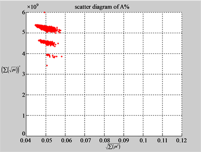
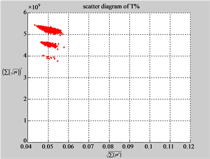
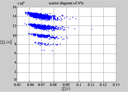
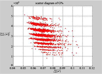
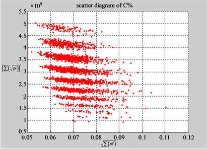
Figure 5. Two groups of eight 2D maps in the range of n = 15, k = 7, N  200 ~ 600, T = 2700; (a) group (a1 - a4) four MapV maps for the file right; (b) group (b1 - b4) four MapV maps for the file 201 - 500.
 (a1) MapA (a2) MapT
 (b1) MapA (b2) MapT
 (a3) MapG (a4) MapC
 (b3) MapG (b4) MapC
 (c1) MapA (c2) MapT

 (d1) MapA (d2) MapT
 (c3) MapG (c4) MapC
 (d3) MapG (d4) MapC
 (e1) MapA (e2) MapT

 (f1) MapA (f2) MapT
 (e3) MapG (e4) MapC

 (f3) MapG (f4) MapC
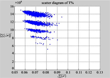
Figure 6. Six groups of twenty six 2D maps in the range of n = 12, k = 7, N = 500, T = 2700 for the file hc256, r = {1,2, 3}, mode = {1,2}; (a1 - 4) Four maps for the file hc256, r = 1, mode = 1; (b1 - 4) Four maps for the file hc256, r = 1, mode = 2; (c1 - 4) Four maps for the file hc256, r = 2, mode = 1; (d1 - 4) Four maps for the file hc256, r = 2, mode = 2; (e1 - 4) Four maps for the file hc256, r = 3, mode = 1; (f1 - 4) Four maps for the file hc256, r = 3, mode = 2.

 MapA (a1) (b1) (c1)

 MapA (d1) (e1) (f1)

 MapT (a2) (b2) (c2)
 MapT (d2) (e2) (f2)
 MapG (a3) (b3) (c3)
 MapG (d3) (e3) (f3)
 MapC (a4) (b4) (c4)
 MapC (d4) (e4) (f4)
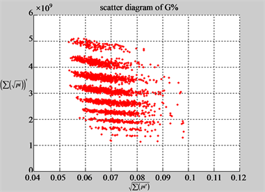
Figure 7. Six groups of twenty-four maps in the ranges: N = 500, T = 2700, k = 7; (a) (f) Real DNA Data; (a1 - 4) DNA sequences from the file right, n = 15, mode = 0; (b - e) Simulation Data; (b1 - 4) Binary Sequences from the file hc256, n = 12, r = 1, mode = 1; (c1 - 4) Binary Sequences from the file hc256, n = 12, r = 3, mode = 1; (d1 - 4) Binary Sequences from the file hc256, n = 12, r = 1, mode = 2; (e1 - 4) Binary Sequences from the file hc256, n = 12, r = 3, mode = 2; (f1 - 4) DNA sequences from the file 201 - 500, n = 15, mode = 0.
potentially contained in DNA sequences. Selected parameters are in the range of . Group (a) provides four
  maps (a1 - a4) for the file right; group (b) uses four
  maps (b1 - b4) for the file 201 - 500.
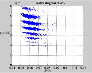
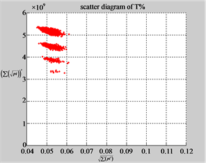
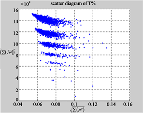
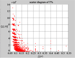
In convenient description, let ~ be a similar operator, for groups (a) & (b), four pairs of {(a1) ~ (a2), (a3) ~ (a4), (b1) ~ (b2) ~ (b3) ~ (b4)} maps i.e. (right-A ~ right-T, right-C ~ right-G, 201-500-A ~ 201-500-T ~ 201-500-C ~ 201-500-C). Two sets of maps have a stronger similar distribution among their projections. From a symmetric viewpoint, three clustering classes could be identified as {(a1) ~ (a2), (a3) ~ (a4), (b1) ~ (b2) ~ (b3) ~ (b4)} respectively. This type of similar clustering distributions may strongly indicate eight maps with intrinsically higher levels of DNA sequences with clear A-T & G-C pairs of symmetric relationships on right for noncoding sequences. And another set of four maps may have similar distributions for coding sequences.
Using a set of selected parameters, six groups of twenty four 2D maps are listed in Figure 6 for the file hc256, r = {1, 2, 3}, mode = {1,2} to explore properties for their higher levels of structures potentially contained in pseudo DNA sequences. Selected parameters are in the range of . Groups (a) - (b) for r = 1 provide two sets of four MapV maps(a1 - a4) mode = 1, (b1 - b4) mode = 2; groups (c) - (d) for r = 2 uses two sets of four
  maps (c1 - c4) mode = 1, (d1 - d4) mode = 2; groups (e) - (f) for r = 3 use two sets offour MapV maps (e1 - e4) mode = 1, (f1 - f4) mode = 2. Using a similar operator, for groups (a - f), following relations are identified {(a1) ~ (c1) ~ (e1) ~ (a2) ~ (c2) ~ (e2), (a3) ~ (c3) ~ (e3) ~ (a4) ~ (c4) ~ (e4), (b1) ~ (d1) ~ (f1) ~ (b2) ~ (d2) ~ (f2) ~ (b3) ~ (d3) ~ (f3) ~ (b4) ~ (d4) ~ (f4)} maps for A ~ T, G ~ C (mode = 1) and A ~ T ~ G ~ C (mode = 2). i.e. three sets of maps are shown in (A ~ T, G ~ C) and another three sets of maps are shown in (A ~ T ~ G ~ C) respectively.
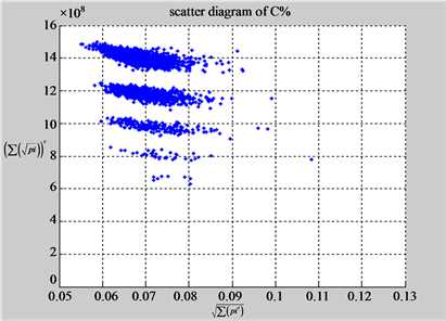
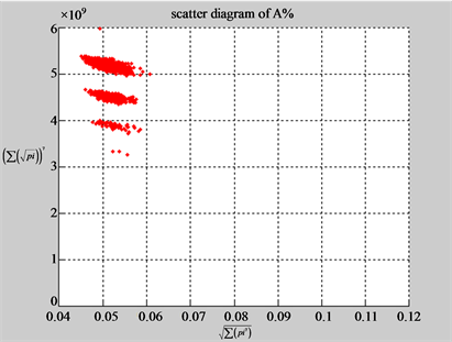
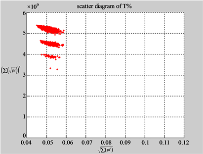
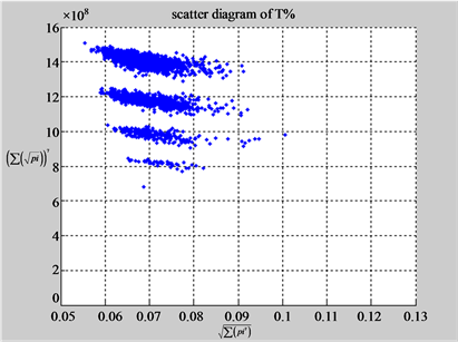
In a convenient comparison, using a set of selected parameters, six groups of twenty four 2D maps are compared in Figure 7 for the files: right, 201 - 500 and hc256, r = {1,3}, mode = {1,2} from (a) - (f) to check their distribution properties contained in both DNA and created pseudo DNA sequences. Group (a) provides four MapV maps (a1 - a4) for the file right; groups (b) and (c) for hc256, mode = 1 provide four  maps (b1 - b4) for r = 1 and (c1 - c4) for r = 3; groups (d) and (e) for hc256, mode = 2 provide four
  maps (d1 - d4) for r = 1 and (e1 - e4) for r = 3. Group (f) provides four
  maps (f1 - f4) for the file 201 - 500.
Using a similar operator , for groups (a - f), four pairs of {(a1)
  (a2), (a3) ~ (a4), (b1)
  (b2), (b3) ~ (b4), (c1) ~ (c2), (c3) ~ (c4), (d1) ~ (d2) ~ (d3) ~ (d4), (e1) ~ (e2) ~ (e3) ~ (e4), (f1) ~ (f2) ~ (f3) ~ (f4)} maps have similar distributions among maps. i.e. Three groups’ maps are shown in relationships among (A ~ T,G ~ C) for non-coding sequences and pseudo DNA sequences on mode = 1 condition and another three groups are shown in the relationships on (A ~ T ~ G ~ C)for coding sequences and pseudo DNA sequences on mode = 2 condition respectively.
In general, this set of map results illustrates directly visual comparisons with similarity between real DNA and pseudo DNA sequences on PDVM maps, their similarly clustering distributions may indicate those simulation results with comparable mechanism to analogy complex behaviors of real DNA sequences with extra A-T & G-C pairs of symmetric relationships or A-T-G-C equal distributions in their higher levels of relationships applying the Stream Cipher mechanism.
5. Conclusion
This paper proposes the architecture to support the Pseudo DNA Variant Map on Cellular Automata. Using a binary random sequence as input, a set of special pseudo DNA sequences can be generated. Under variant measures, probability measurement and normalized histogram, a pair of values can be determined by a series of controlled parameters. Collecting relevant pairs on multiple DNA sequences, four 2D maps can be generated.
The main results of this paper provide the PDVM architecture description in diagrams, main components, modules, expressions and important equations for the PDVM. Core models and diagrams, sample results are illustrated to apply two types of data sets selected from real DNA sequences and two types of controllable modes to generate relevant pseudo random sequences from the Stream Cipher HC-256 for comparison under the PDVM testing. After the proper set of parameters selected, suitable visual distributions could be observed using the PDVM. Results in Figures 4-7 provide useful evidences systematically to support proposed PDVM useful in checking higher levels of symmetric/similar properties among complex DNA sequences in both natural and the artificial environment.
This construction could provide useful insights to simulate spatial information on complex DNA expressions especially on both large non-coding and coding RNA/DNA construction via 2D maps to explore higher levels of complex interactive environments using Cellular Automata schemes in near future.
Acknowledgements
Thanks to Weiqiong Zhang for generating maps, Ruoyu Shen for generating HC-256 pseudo DNA sequences, to the school of software Yunnan University, the key laboratory of Yunnan software engineering and the key laboratory for Conservation and Utilization of Bio-resource for excellent working environment, to the Yunnan Advanced Overseas Scholar Project (W8110305), the Key R&D project of Yunnan Higher Education Bureau (K1059178) and National Science Foundation of China (61362014) for financial supports to this project.
Funding
Project supported by NSF of China (61362014), the Key R&D project of Yunnan Higher Education Bureau (K1059178) and Yunnan Advanced Overseas Scholar Project (W8110305).
REFERENCES
- M. Santha and U. V. Vazirani, “Generating Quasi-Random Sequences from Slightly Random Sources,” Journal of Computer and System Sciences, Vol. 33, No. 1, 1986, pp. 75-87. http://dx.doi.org/10.1016/0022-0000(86)90044-9
- G. B. Agnew, “Random Source for Cryptographic Systems,” Advanced in Cryptology—EUROCRYPT’87 Proceedings, SpringerVerlag, Berlin, 1988, pp. 77-81.
- M. Schoöniger and A. von Haeseler, “Simulating Efficiently the Evolution of DNA Sequences,” Bioinformatics, Vol. 11, No. 1, 1995, pp. 111-115. http://dx.doi.org/10.1093/bioinformatics/11.1.111
- A. Gehani, T. LaBean and J. Reif, “DNA-Based Cryptography,” DIMACS Series in Discrete Mathematica and Theoretical Computer Science, Vol. 54, 2000, pp. 233-249. http://www.cs.duke.edu/~reif/paper/DNAcrypt/DNA5.DNAcrypt.pdf
- eSTREAM Project, 2012. http://en.wikipedia.org/wiki/ESTREAM
- H. J. Wu, “Stream Cipher HC-256,” ESTREAM, 2004. http://www.ecrypt.eu.org/stream/p3ciphers/hc/hc256_p3.pdf
- F. Piva and G. Principato, “RANDNA: A Random DNA Sequence Generator,” Silico Biology, Vol. 6, 0024, 2006. http://www.bioinfo.de/isb/2006060024/
- E. Lieberman-Aiden, et al., “Comprehensive Mapping of Long-Range Interactions Reveals Folding Principles of the Human Genome,” Science, Vol. 326, No. 5950, 2009, pp. 289-293. http://dx.doi.org/10.1126/science.1181369
- A. Arneodo, C. Vaillant, B. Audit, F. Argoul. Y. d’Aubenton-Carafa and C. Thermes, “Multi-Scale Coding of Genomic Information: From DNA Sequence to Genome Structure and Function,” Physics Reports, Vol. 498, No. 2-3, 2011, pp. 45-188. http://dx.doi.org/10.1016/j.physrep.2010.10.001
- S. Engela, A. Alemany, N. Forns, P. Maass and F. Ritort, “Folding and Unfolding of a Triple-Branch DNA Molecule with Four Conformational States,” Philosophical Magazine, Vol. 91, No. 13-15, 2011, pp. 2049-2065. http://dx.doi.org/10.1080/14786435.2011.557671
- H. Y. Zhang and X. Y. Liu. “A CLIQUE Algorithm Using DNA Computing Techniques Based on Closed-Circle DNA Sequences,” Biosystems, Vol. 105, No. 1, 2011, pp. 73-82. http://dx.doi.org/10.1016/j.biosystems.2011.03.004
- B. Banfai, H. Jia, J. Khatun, et al., “Long Noncoding RNAs Are Rarely Translated in Two Human Cell Lines,” Genome Research, Vol. 22, 2012, pp. 1646-1657. http://dx.doi.org/10.1101/gr.134767.111
- M. B. Gerstein, A. Kundaje, M. Hariharan, et al., “Architecture of the Human Regulatory Network Derived from ENCODE Data,” Nature, Vol. 489, No. 7414, 2012, pp. 91-100. http://dx.doi.org/10.1038/nature11245
- B. E. Bernstein, E. Birney, I. Dunham, et al., “An Integrated Encyclopedia of DNA,” Nature, Vol. 489, No. 7414, 2012, pp. 57-74. http://dx.doi.org/10.1038/nature11247
- E. Pennisi, “Genomics. ENCODE Project Writes Eulogy for Junk DNA,” Science, Vol. 337, No. 6099, 2012, pp. 1159-1161. http://dx.doi.org/10.1126/science.337.6099.1159
- W. F. Doolittle, “Is Junk DNA bunk? A Critique of ENCODE,” Proceedings of the National Academy of Sciences of the United States of America, Vol. 110, 2013, pp. 5294-5300.
- J. M. Engreitz, A. Pandya-Jones, P. McDonel, et al., “Large Noncoding RNAs can Localize to Regulatory DNA Targets by Exploriting the 3D Architecture of the Genome,” Cold Spring Harbor Laboratory Press, Proceedings of The Biology of Genomes, 2013, p. 122.
- J. S. Wang and M. Yan, “Numerical Methods in Bioinformatics,” Science Press, Beijing, 2013.
- C. M. Gearheart, B. Arazi and E. C. Rouchka, “DNA-Based Random Number Generation in Security Circuitry,” Biosystems, Vol. 100, No. 3, 2010, pp. 208-214. http://dx.doi.org/10.1016/j.biosystems.2010.03.005
- O. Okunoye Babatunde. “On Pseudorandom Number Generation from Programmable and Computable Biomolecules: Deoxyribonucleic (DNA) as a Novel Pseudorandom Number Generator,” World Applied Programming, Vol. 1, No. 3, 2011, pp. 215-227.
- Y. P. Zhang, Y. Zhu, Z. Wang, R. O. Sinnott, “Index-Based Symmetric DNA Encryption Algorithm,” 4th International Congress on Image and Signal Processing (CSIP), Shanghai, 2011, pp. 2290-2294. http://dtl.unimelb.edu.au/researchfile287042.pdf
- Y. P. Zhang and L. H. Bochen Fu (2012). “Research on DNA Cryptography,” In: J. Sen, Ed., Applied Cryptography and Network Security, InTech Press, Rijeka, Croatia, 2012, pp. 357-376 http://www.intechopen.com/books/applied-cryptography-and-network-security/research-on-dna-cryptography
- G. C. Sirakoulis. “Hybrid DNA Cellular Automata for Pseudorandom Number Generation,” 2012 International Conference on High Performance Computing and Simulation (HPCS), Madrid, 2-6 July 2012, pp. 238-244
- N. A. Tchurikov, O. V. Kretova, D. M. Fedoseeva, et al., “DNA Double-Strand Breaks Coupled with PARP1 and HNRNPA2B1 Binding Sites Flank Coordinately Expressed Domains in Human Chromosomes,” PLoS Genetics, Vol. 9, No. 4, 2013, Article ID: e1003429. http://dx.doi.org/10.1371/journal.pgen.1003429
- J. Z. J. Zheng and C. H. Zheng, “A Framework to Express Variant and Invariant Functional Spaces for Binary Logic,” Frontiers of Electrical and Electronic Engineering in China, Vol. 5, No. 2, 2010, pp. 163-172. http://www.springerlink.com/content/91474403127n446u/
- J. Zheng, C. Zheng and T. Kunii, “A Framework of Variant Logic Construction for Cellular Automata,” In: A. Salcido, Ed., Cellular Automata—Innovative Modelling for Science and Engineering, InTech Press, Rijeka, Croatia, 2011, pp. 325-352. http://www.intechopen.com/chapters/20706
- Q. P. Li and J. Zheng, “2D Spatial Distributions for Measures of Random Sequences Using Conjugate Maps,” The Proceedings of the 11th Australian Information Warfare and Security Conference, Perth, 30 November-2 December 2010, pp. 1-9. http://ro.ecu.edu.au/isw/34
- J. Zheng, C. Zheng and T, Kunii, “Interactive Maps on Variant Phase Spaces—From Measurements-Micro Ensembles to Ensemble Matrices on Statistical Mechanics of Particle Models,” In: A. Salcido, Ed., Emerging Application of Cellular Automata, InTech Press, Rijeka, Croatia, 2013, pp. 113-196. http://dx.doi.org/10.5772/51635
- J. Zheng, “Novel Pseudo-Random Number Generation Using Variant Logic Framework,” 2nd International Cyber Resilience Conference, 2011, pp. 100-104. http://igneous.scis.ecu.edu.au/proceedings/2011/icr/zheng.pdf
- W. Z. Yang and J. Zheng, “Pseudo-Random Number Generator Based on Variant Logic Model,” ChinaCom 2012 Conference Proceedings, 2012.
- W. Z. Yang and J. Zheng, “Variant Pseudo-Random Number Generator,” Hakin9 Extra, Vol. 6, No. 13, 2012, pp. 28-31. http://hakin9.org/hakin9-extra-62012/
- W. Q. Zhang and J. Zheng, “Randomness Measurement of Pseudorandom Sequence Using different Generation Mechanisms and DNA Sequence,” Journal of Chengdu University of Information Technology, Vol. 27, No. 6, 2012, pp. 548-555.
- J. Zheng, W. Q. Zhang, J. Luo, W. Zhou and R. Shen, “Variant Map System to Simulate Complex Properties of DNA Interactions Using Binary Sequences,” Advances in Pure Mathematics, Special Issue: Number Theory and Cryptology, Vol. 3, No. 7A, 2013, pp. 5-24.
NOTES

*Corresponding author.