Applied Mathematics
Vol. 4 No. 8 (2013) , Article ID: 35589 , 5 pages DOI:10.4236/am.2013.48165
Riemann Boundary Value Problem of Non-Normal Type on the Infinite Straight Line
Department of Information and Computing Sciences, Mathematics College, Northeast Petroleum University, Daqing, China
Email: caolixia98237@163.com
Copyright © 2013 Lixia Cao. This is an open access article distributed under the Creative Commons Attribution License, which permits unrestricted use, distribution, and reproduction in any medium, provided the original work is properly cited.
Received June 16, 2013; revised July 16, 2013; accepted July 25, 2013
Keywords: Non-Normal Type; Riemann Boundary Value Problem; The Infinite Straight Line
ABSTRACT
We consider a Riemann boundary value problem of non-normal type on the infinite straight line. By using the method of complex functions, we investigate the method for solving this Riemann boundary value problem of non-normal type and give the general solutions and the solvable conditions for it.
1. Introduction
Various kinds of Riemann boundary value problems (BVPs) for analytic functions on closed curves or on open arc, doubly periodic Riemann BVPs, doubly quasi-periodic Riemann BVPs, and BVPs for polyanalytic functions have been widely investigated in [1-8]. The main approach is to use the decomposition of polyanalytic functions and their generalization to transform the boundary value problems to their corresponding boundary value problems for analytic functions. Recently, inverse Riemann BVPs for generalized analytic functions or bianalytic functions have been investigated in [9-12].
In this paper, we consider a kind of Riemann BVP of non-normal type on the infinite straight line and discuss the solvable conditions and the general solution for it.
2. A Riemann Boundary Value Problem of Non-Normal Type on the Infinite Straight Line
Let  be the real axis oriented in the positive direction. And let
 ,
,  denote the upper half-plane and the lower half-plane cut by
 . Our objective is to find a sectioally holomorphic function
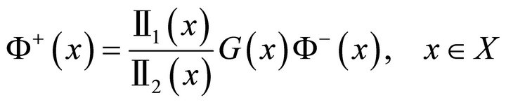
  satisfying the following boundary condition
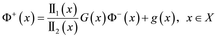 (1)
(1)
where the two given functions  and
and on
on  with
with  existing and
  (clearly
  exists), and
 ,
,  with
with

being on  and
and . And the integer
is the index of problem (1).
Write
 .
.
Without loss of generality, we can consider problem (1) in class , that is, the two limits
  and
and  exist as
 . Clearly, here we have
 .
.
3. Homogeneous Problem
The homogeneous problem of (1) is as follows
 . (2)
. (2)
It is found that  is required for solving problem (2) in class
 . Here we suppose that
 . Let
. Let
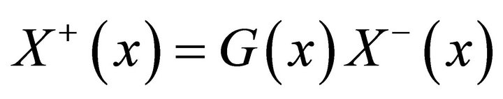
 , (3)
, (3)
then  and
and  with
with
 and
and
 . (4)
. (4)
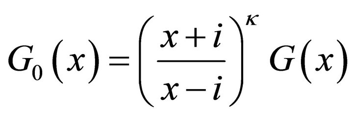
Write
 . (5)
. (5)
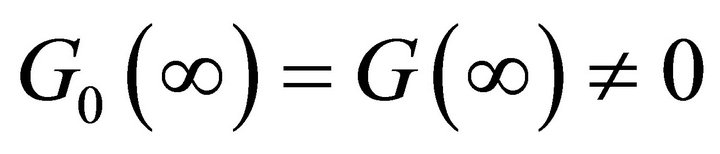
Since , by taking logarithm of
  for some branch we obtain a single-valued function
  with
with , hence
  exists with
  and
and . And by simple calculation we see that
  is sectionally holomorphic.
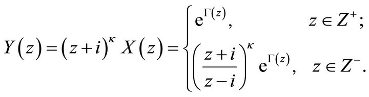
Write
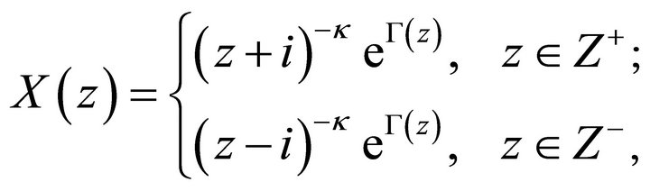 (6)
(6)
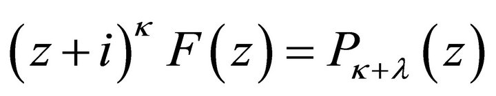
then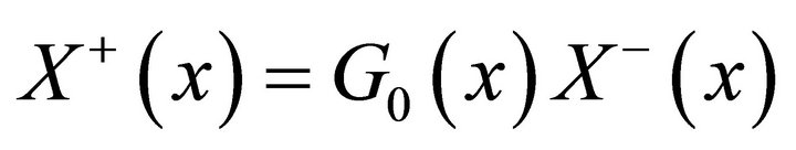 . Substituting this into (2) gives
 .
.
If we write
then we get . Thus
  is analytic on the whole complex plane and has at most
  order at
 . From [5], we know that
  must be an arbitrary polynomial
  of degree
  with
with  if
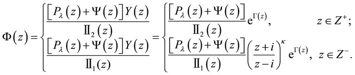
if . Therefore, the homogeneous problem (2) has general solution in class
  as follows
 (7)
(7)
Considering the requirements that  and
and  are bounded at
 we can let
 where
where  is an arbitrary polynomial of degree
  with
with  if
if . Now we get the general solution in class
  for the homogeneous problem (2) as follows
 (8)
(8)
Thus we get the following results.
Theorem 3.1. For the homogeneous problem (2) in class , the following two cases arise.
1) When , it is always solvable and its general solution is given by (8), where
  is an arbitrary polynomial of degree
 .
.
2) When , it only has zero-solution.
4. Nonhomogeneous Problem
For nonhomogeneous problem (1), the key is to find out the special solution.
Similar to the case in homogeneous problem (2), the canonical function  is given by (6) but with
satisfying
 .
.
By this, problem (1) can be rewritten as
 (9)
(9)
We note that Plemelj formula can not be used directly here, because that when 
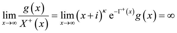
is not a finite constant, and so 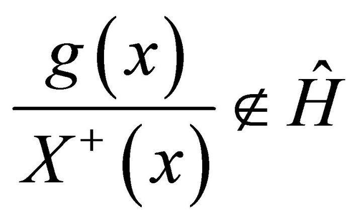 (unless
 ). For a unified treatment, regardless of the value of
 , we always let
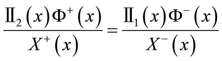
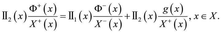
Multiplying  to the two sides of (9) gives
 .
.
We know that  and so that
 .
.
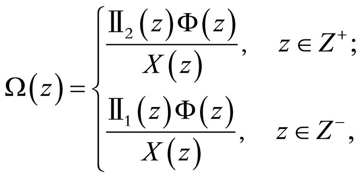
If we let
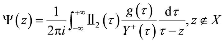 , (10)
then we get
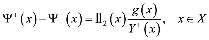 and
and
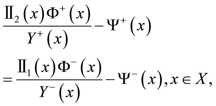 (11)
(11)
with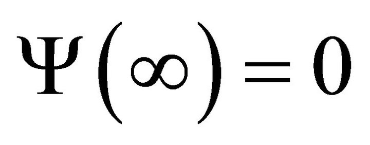 . Similar to the reasoning for (7) for problem (2), we know that if problem (1) has solution in class
 , then can easily write out the form. But for problem (11), the function
is analytic everywhere except at the possible unique pole , therefore the following two cases arise.
Case 1. .
.
When ,
,  has a pole of order
  at
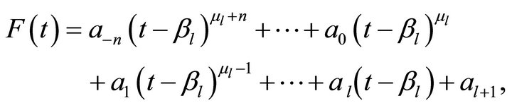
at . To eliminate the singularity, we multiply
  to
to  and get a polynomial of degree
 :
:
 .
.
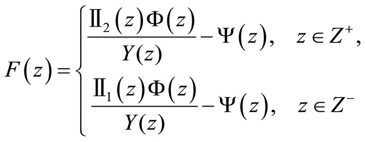
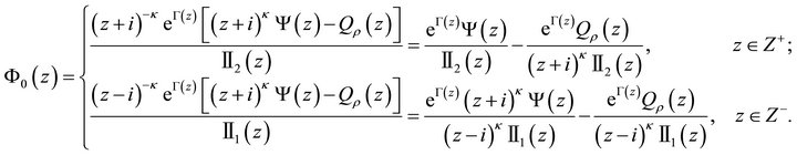
Therefore
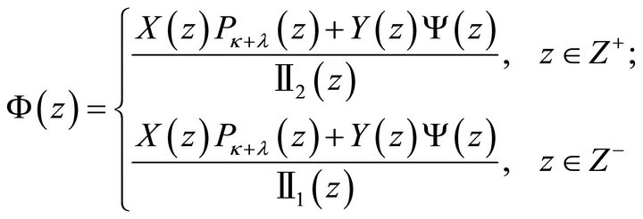 (12)
(12)
is actually the general solution for problem (1) in class , where
 . For convenience, we deform the function
  given by (12) into
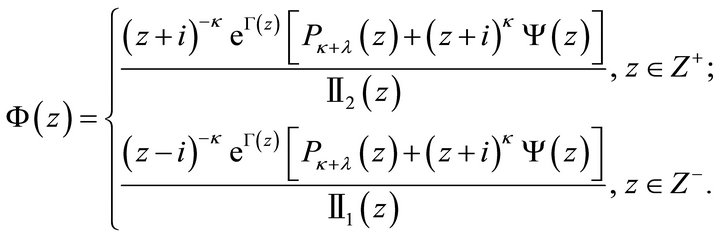 (13)
(13)
Considering the requirements that  are bounded on
 , and the fact that
with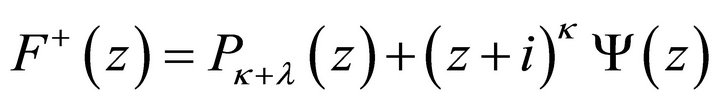 , the smallest degree of
  in the numerator of the above formula should be
 , we suppose that
then when , we have
and the smallest degree of  in numerator is
  (i.e.
(i.e.  is bounded on
 ) only when
 that is,
 (14)
(14)
In a similar way, we know that  is bounded on
  only when
 (15)
(15)
are satisfied.
Hence, we get the results that  are bounded on
  only when the conditions (14) and (15) are all satisfied. While it is troublesome to solve the system composed by (14) and (15) for the coefficients of
 .
.
Here we aim to determine the coefficients by using Hermite interpolation polynomial.
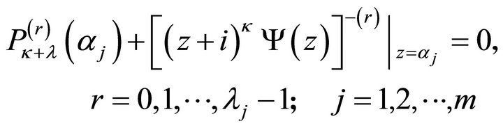
Firstly, we make the polynomial  of degree
 such that


The polynomial  exists uniguely from [5]. Let
 (16)
(16)
We can see from (16) that  are continuous on
 , and through simple verification that
  satisfy the condition in problem (1), and that the order of
  at
at  is
is .
.
Now we aim to make  belong to
  by adding restricted conditions.
a) If , that is,
  ,
,  exactly belongs to
  and is justly the solution for homogeneous problem of (2), and also a particular solution for nonhomogeneous problem (1) in
 . Combining with the general solution (8) of homogeneous problem (2), we known that when
 , the general solution of problem (1) in
  is
is
 (17)
(17)
where  when
when .
.
b) If , that is,
  , since the homogeneous problem (2) corresponding to (1) only has zero-solution in
 , the existence of a solution
  for nonhomogeneous problem (1) in
  implies the uniqueness. Because
  has generally singularity of order
  at
at ,
,  belongs to
  if and only if
  conditions on
  or on
or on  are satisfied.
By rewriting  as
as
Here we write
 . (18)
Since the order of the denominator in  is
is 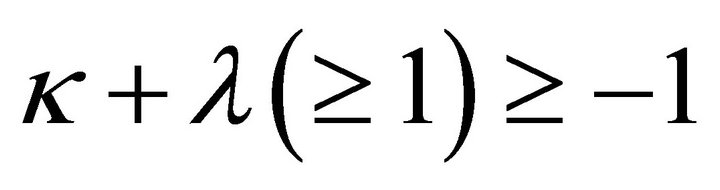 (is always true), it is enough that
  is at most a polynomial of degree
 , that is,
 . (19)
Therefore, only when condition (19) is satisfied, (16) is actually the general solution for nonhomogenous problem (1), now the homogeneous problem (2) only has zero-solution.
Case 2. .
.
When ,
,  is analytic on the whole complex plane and has
  order at
 , that is,
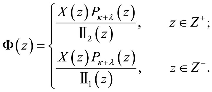
  , and now the homogeneous problem (2) only has zero-solution. Therefore the general solution for nonhomogenous problem (1) in
  is given by
 (20)
(20)
If we make the Hermite interpolation polynomial of degree , the fact that
  (the order of the denominator) implies that
  is unbounded on
 , which contradicts with the hypothesis that
  is bounded on
 . So it is infeasible to make the Hermite interpolation polynomial for this.
However, we have the following effective treatment for this.
a) Under this situation,  may have the unique pole at
 . In order to eliminate the pole, we should put the following restrictions for it:
if , we only need
 ; (21)
if , we only need to put
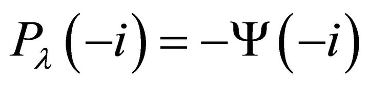 ; (22)
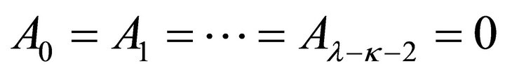
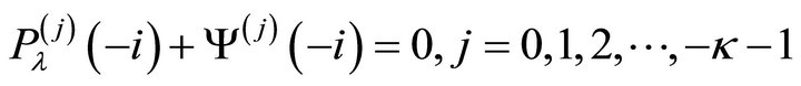
if , apart from (22), the restrictions
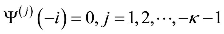 or
or
 (23)
(23)
are necessary.
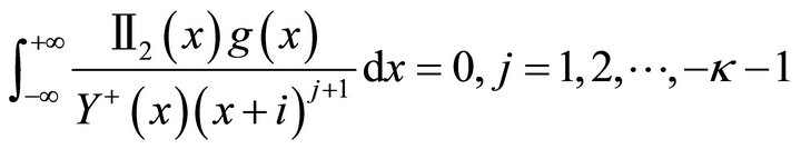
b) Considering the boundedness of  on
on , the following restrictions are also necessary:
 (24)
(24)
 (25)
(25)
Thus we get the following results.
Theorem 4.1. For the nonhomogeneous problem (1) in class , the following two cases arise.
1) . If
. If , problem (1) is always solvable and its general solution is given by (17); and if
 , if and only if
  satisfies condition (19), problem (1) has unique solution, given by (16).
2) When , it has unique solution in form (20) when the restrictions (21) or (22) or (22)-(23), and (24)- (25) are satisfied.
Anyway, the degree of freedom of solution for nonhomogeneous problem (1) is .
.
REFERENCES
- M. B. Balk, “Polyanalytic Functions,” Akademie Verlag, Berlin, 1991.
- H. Begehr and A. Kumar, “Boundary Value Problems for the Inhomogeneous Polyanalytic Equation I,” Analysis: International Mathematical Journal of Analysis and Its Application, Vol. 25, No. 1, 2005, pp. 55-71.
- D. Jinyuan and W. Yufeng, “On Boundary Value Problems of Polyanalytic Functions on the Real Axis,” Complex Variables, Vol. 48, No. 6, 2003, pp. 527-542. doi:10.1080/0278107031000103412
- B. F. Fatulaev, “The Main Haseman Type Boundary Value Problem for Metaanalytic Function in the Case of Circular Domains,” Mathematical Modelling and Analysis, Vol. 6, No. 1, 2001, pp. 68-76.
- J. K. Lu, “Boundary Value Problems for Analytic Functions,” World Scientific, Singapore City, 1993.
- A. S. Mshimba, “A Mixed Boundary Value Problem for Polyanalytic Function of Order n in the Sobolev Space Wn, p(D),” Complex Variables, Vol. 47, No. 12, 2002, pp. 278-1077.
- N. I. Muskhelishvili, “Singular Integral Equations,” World Scientific, Singapore City, 1993.
- W. Yufeng and D. Jinyuan, “Hilbert Boundary Value Problems of Polyanalytic Functions on the Unit Circumference,” Complex Variables and Elliptic Equations, Vol. 51, No. 8-11, 2006, pp. 923-943. doi:10.1080/17476930600667692
- L. Xing, “A Class of Periodic Riemann Boundary Value Inverse Problems,” Proceedings of the Second Asian Mathematical Conference, Nakhon Ratchasima, 17-20 October 1995, pp. 397-400.
- M. H. Wang, “Inverse Riemann Boundary Value Problems for Generalized Analytic Functions,” Journal of Ningxia University of Natural Resources and Life Sciences Education, Vol. 27, No. 1, 2006, pp. 18-24.
- X. Q. Wen and M. Z. Li, “A Class of Inverse Riemann Boundary Value Problems for Generalized Holomorphic Functions,” Journal of Mathematical, Vol. 24, No. 4, 2004, pp. 457-464.
- L. X. Cao, P.-R. Li and P. Sun, “The Hilbert Boundary Value Problem With Parametric Unknown Function on Upper Half-Plane,” Mathematics in Practice and Theory, Vol. 42, No. 2, 2012, pp. 189-194.