Applied Mathematics
Vol.4 No.4(2013), Article ID:30767,5 pages DOI:10.4236/am.2013.44099
Exact Solution of Terzaghi’s Consolidation Equation and Extension to Two/Three-Dimensional Cases
Wizard Technology, Teramo, Italy
Email: romolo.difrancesco@vodafone.it
Copyright © 2013 Romolo Di Francesco. This is an open access article distributed under the Creative Commons Attribution License, which permits unrestricted use, distribution, and reproduction in any medium, provided the original work is properly cited.
Received January 25, 2013; revised February 28, 2013; accepted March 5, 2013
Keywords: Terzaghi; One-Dimensional Consolidation; Pore Overpressure; Two/Three-Dimensional Consolidation
ABSTRACT
The differential equation by Terzaghi and Fröhlich, better known as Terzaghi’s one-dimensional consolidation equation, simulates the visco-elastic behaviour of soils depending on the loads applied as it happens, for example, when foundations are laid and start carrying the weight of the structure. Its application is traditionally based on Taylor’s solution that approximates experimental results by introducing non-dimensional variables that, however, contradict the actual behaviour of soils. The proposal of this research is an exact solution consisting in a non-linear equation that can be considered correct as it meets both mathematical and experimental requirements. The solution proposed is extended to include differential equations relating to two/three dimensional consolidation by adopting a transversally isotropic model more consistent with the inner structure of soils.
1. Introduction
The mechanical behaviour of soils was coded only after the introduction of the “concept of effective stresses” [1] which marked the birth of Soil Mechanics starting from the general structure of Continuum Mechanics from which it derives. This concept is based on the inner structure of soils that are composed of a solid skeleton and inter-particle gaps. These pores are more or less interconnected and through them run fluids of different nature. Therefore, in view of a necessary simplification of the mathematics of associated phenomena, the concept of effective stresses requires the soils to be assimilated to bi-phasic systems composed of a solid skeleton saturated with water, i.e. two continuous means that act in parallel and share the stress status:
 . (1)
. (1)
In Equation (1) there is the tensor of the total stresses exerted by the solid skeleton , the hydrostatic pressure exerted by the fluid (u0, known as interstitial pressure) and Kronecker’s delta
 ; furthermore, from a merely phenomenological point of view, Equation (1) attributes the soil shear resistance only to effective stress, independent of the presence of the fluid.
It should be highlighted that the concept of effective stresses is valid only in stable conditions, when the fluid is in balance with the solid skeleton. In these conditions you can calculate the hydrostatic component in all points of the underground and in all moments through the application of the laws of balance; vice-versa, i + n transient conditions, it is necessary to introduce other elements capable of accounting for the variation of the component u0 induced by stresses of various nature.
At this point, the problem focus is on the permeability coefficient (K = m/sec) that, by expressing the capacity of a soil to transmit a fluid, takes on the character of a velocity and varies approximately in the range 10–1/10–10 m/sec depending on the inner structure of the solid skeleton. As a direct consequence of this extreme variability, the soils with high permeability (such as sands) behave as open hydraulic systems where compression induced, for example, by the load of a foundation, causes simultaneous drainage of the fluid from the pores. In practice, the fluid does not take part in the mechanical response and the stress induced weighs only on the solid skeleton that, in turn, subsides in association with reduced porosity. On the contrary, soils with very low permeability (such as clays) exhibit hydraulic delay in reacting to stresses, with consequent development of an initial interstitial overpressure  that contradicts Equation (1), and participate in the mechanical response with the solid skeleton. A transient filtering motion follows that comes to end only when the initial value of the interstitial pressure is reset
 .
.
In practice, given that a deformation of the solid skeleton occurs together with the expulsion of water, sands develop elasto-plastic settlements synchronous with load application while clays exhibit time-dependent consolidation settlements typically characterized as reverse hyperbolic functions.
Considering the above, the one-dimensional consolidation equation [1,2] describes the hydraulic behaviour of soils in transient conditions by making it possible to simulate the variation in time of interstitial overpressures (ue), generated—for example—by the load induced by a foundation or by a road embankment (Figure 1), with consequent visco-elastic settlements to which corresponds a structural reorganisation of the solid skeleton, with reduction of porosity and, concurrently, of the degrees of freedom.
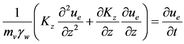
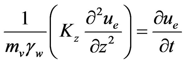
This formulation can be inferred from applying the continuity equation to supposedly saturated soils leading [3], with a few mathematical manipulations, to the following relationship that demonstrates how the transient filtering motion depends on the vertical permeability factor (Kv or Kz), on the compressibility factor (mv) and on the weight of the volume of water (gw = 10 kN/m3) that in turn identifies the fluid:
 . (2)
. (2)
The next step consists in introducing the hypothesis (in contrast with experimental results) that the permeability factor does not change during consolidation:
 . (3)
. (3)
Finally, denoting the consolidation coefficient as cv or cz:
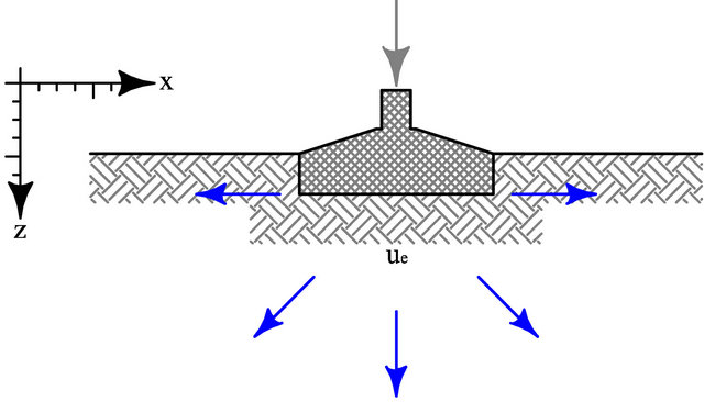
Figure 1. The load transmitted by a foundation always causes interstitial overpressures whose dissipation depends on soil permeability that in turn depends on porosity; consolidation may last from some minutes (loose sands) to tens of years (very stiff clays).
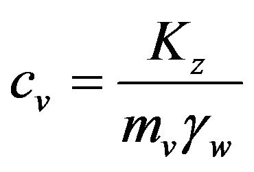 , (4)
, (4)
you come to write the classical one-dimensional consolidation equation:
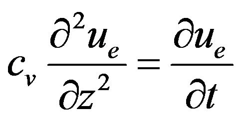 . (5)
. (5)
It should be noticed that Equation (5) is analogous to Fourier’s law on heat propagation to the point that you can define the theory of consolidation as the simulation of the propagation of stress-induced interstitial pressures in the subsoil.
2. Exact Solution of Terzaghi’s Consolidation Equation
2.1. Assumptions
Let’s assume that  are two positive constants assigned and that:
 (6)
(6)
is the regular function given by:
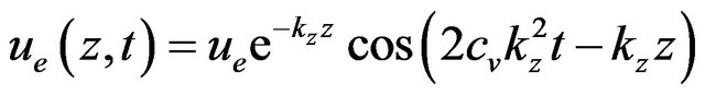 . (7)
. (7)
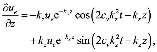
Now, you can easily notice that  solves the differential Equation (5); indeed, given the validity of the following:
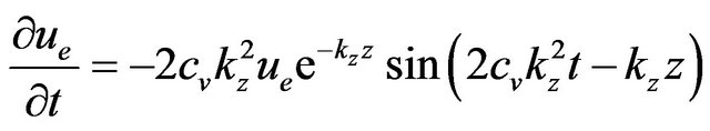 , (8)
, (8)
 (9)
(9)
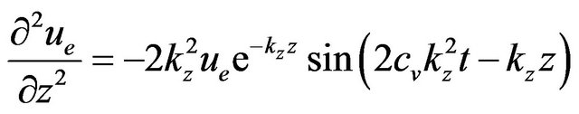 , (10)
you obtain:
 , (11)
which is the differential equation given.
If you analyse function (7), you will find out that it simulates the time variation of interstitial overpressures in the subsoil through the consolidation constant kz— starting from the point where they are triggered—by dampening their width as depth increases through a reverse hyperbolic function.
2.2. Connection with Experimental Data
Now, since function (7) is a solution of Equation (5), it should be necessarily extended also to experimental methods—oedometrically considered—in order to determine the parameters that govern it correctly. In this sense, it may be useful to analyse an important property of the function ue.
Given H > 0 (Figure 2), it can be useful to identify the instant tH > 0 to which the following conditions apply:
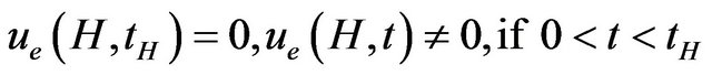 . (12)
As a first passage, you should notice that equation  reduces to the form:
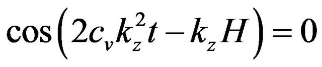 (13)
(13)
which has infinite solutions like:
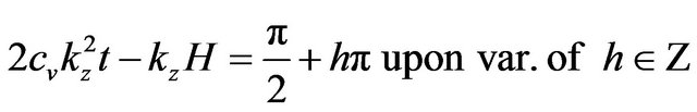 (14)
(14)
or like:
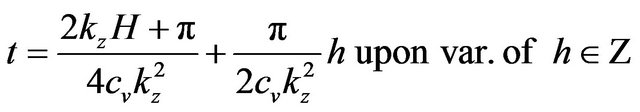 (15)
(15)
The next passage consists in selecting the positive value t closest to zero from among those determined by setting the condition t > 0 that provides:
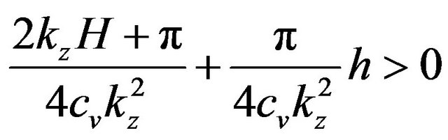 (16)
(16)
from which we obtain:
 . 17)
. 17)
The last passage includes that, if you set also the following condition:
 , (18)
you obtain the formulation of the consolidation completion time:
 . (19)
Finally, from Equation (19) you can extract the consolidation coefficient:
 . (20)
H is from Figure 2, hH º H100 and tH º t50 from Figure 3 while kz depends on the boundary conditions (uniqueness theorem).
3. Extension to the Two/Three-Dimensional Cases
Let’s put  to be positive constants assigned and be:
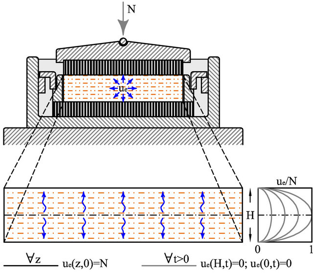
Figure 2. Details of an oedometric cell and indication of the drainage paths [4-7].
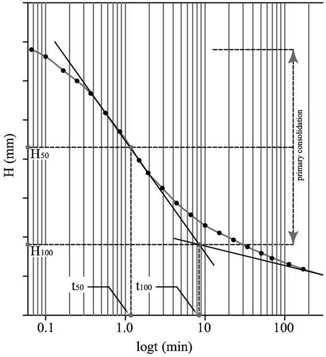
Figure 3. Example of interpretation of a consolidation curve [4-7].
 (21)
(21)
the regular function given by:
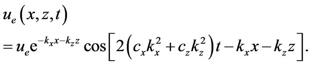 (22)
(22)
Going through the same passages as in Equations (8) to (11), you can easily notice that  solves the differential equation:
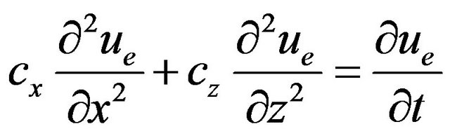 . (23)
Similarly, if  are positive constants assigned and:
 (24)
(24)
the regular function given, then:
 (25)
(25)
solves the differential equation:
 . (26)
4. Conclusions
Notwithstanding that the theory of monodimensional consolidation was first presented in 1936, it is still today taught in all geotechnical engineering courses (for example in Italy: The University of Naples Federico II [8]; The Polytechnic University of Milan [9]; The Polytechnic University of Turin [10]) and is also the only theory used in the professional procedures of engineers and geologists (to predict viscoelastic settlement of ground subjected to loads) and is likewise the only instrument applied in geotechnical laboratories to derive experimental data using oedometric tests.
The only valid alternative is provided by Biot’s theory [11] which is derived from the union of the equation of continuity (3), extended into three dimensions, with Navier’s Equations to produce a system of 4 equations with 4 unknown variables relating to the interstitial pressure and movement along three directions. However owing to its complexity it is only applicable in simple cases, for which a precise solution exists [12-21] or when the solution is arrived at using numeric methods—for example— the finite elements method implemented in modern professional and research software [22,23].
With in mind the entire Mechanics of Soils, and the study of the soil visco-elastic behaviour [1,2] in particular, the application of Terzaghi’s differential equation is historically based on Taylor’s solution [24] that approximates experimental results—limited to the one-dimensional case only—through the introduction of arbitrary and fixed non-dimensional variables, independent of the geological history of the means. This research work makes a proposal for an exact solution that can be considered correct as it solves the differential equation and, at the same time, allow correct interpretation of experimental data; then, solution has been fruitfully extended to the twoand three-dimensional cases.
To conclude, results even satisfactory have come to light from the analysis of data. At the same time, they have opened additional research channels, considering that the uniqueness theorem will be proved later on the basin of the oedometric boundary conditions.
5. Acknowledgements
The author wishes to thank Luca Lussari, Department of Mathematics and Physics of “University of Sacro Cuore of Brescia”—Italy, for his suggestions and observations.
REFERENCES
- K. Terzaghi, “Die Berechnung der Durchlassigkeitsziffer des Tones aus Dem Verlauf der Hidrodynamichen Spannungserscheinungen Akademie der Wissenschaften in Wien,” Mathematish-Naturwissen-Schaftiliche Klasse, Vol. 132, 1923, pp. 125-138.
- K. Terzaghi and O. K. Fröhlich, “Theorie der Setzung von Tonschichte,” Franz Deuticke, Leipzig/Wien, 1936.
- T. W. Lambe and R. W. Whitman, “Soil Mechanics,” John Wiley & Sons, New York, 1969.
- K. Terzaghi, “Principles of Soil Mechanics: I—Phenomena of Cohesion of Clays,” Engineering News-Record, Vol. 95, No. 19, 1925, pp. 742-746.
- A. Casagrande, “Structure of Clay and Its Importance in Foundation Engineering,” Journal of Boston Society of Civil Engineers, Vol. 19, No. 14, 1932, pp. 168-209.
- G. Gilboy, “Improved Soil Testing Methods,” Engineering News Record, 21 May 1936.
- P. C. Rutledge, “Relation of Undisturbed Sampling in Laboratory Testing,” Tr. Am. Soc. C.E., No. 109, 1944.
- C. Viggiani, “Foundations,” Hevelius Editore, Benevento, 1999.
- R. Nova, “Fundamental of Soil Mechanics,” McGrawHill, Milano, 2002.
- R. Lancellotta, “Geotechnical,” 3rd Edition, Zanichelli Editore, Bologna, 2004.
- M. A. Biot, “General Theory of Three-Dimensional Consolidation,” Journal of Applied Physics, Vol. 12, No. 2, 1941, pp. 155-164.
- M. A. Biot and F. M. Clingan, “Consolidation Settlement of Soil with an Impervious to Surface,” Journal of Applied Physics, Vol. 12, No. 7, 1941, pp. 578-581.
- J. Mandel, “Consolidation des Couches d’Argille,” Proc. IV ICSMFE, London, 1957.
- J. De Jong, “Application of Stress Function to Consolidation Problems,” Proc. IV ICSMFE, London, 1957.
- R. E. Gibson and J. McNamee, “The Consolidation Settlement of a Load Uniformly Distributed over a Rectangular Area,” Proc. IV ICSMFE, London, 1957.
- J. McNamee and R. E. Gibson, “Plane Strain and Axially Symmetric Problems of the Consolidation of a Semi Infinite Clay Stratum,” Quarterly Journal of Mechanics and Applied Mathematics, Vol. 13, No. 2, 1960, pp. 210-217.
- J. Mandel, “Tassements Produits par la Consolidation d’une Couche d’Argille de Grande Epaisseur,” Proc. V ICSMFE, Paris, 1961.
- C. W. Cryer, “A Comparison of the 3-Dimensional Theories of Biot and Terzaghi,” Quarterly Journal of Mechanics and Applied Mathematics, Vol. 16, 1963, pp. 401-412.
- R. L. Schiffman and A. Fungaroli, “Consolidation Due to Tangential Loads,” Proc. VI ICSMFE, Montreal, 1965.
- R. E. Gibson, J. K. L. Schiffman and S. L. Pu, “Plain Strain and Axially Symmetric Consolidation of a Clay Layer of Limited Thickness,” University of Illinois, Mate Report, 1967, pp. 67-74.
- R. L. Schiffman, A. T. F. Chen and J. C. Jordan, “An Analisys of Consolidation Theories,” Proceedings of the American Society of Civil Engineers, Vol. 98, No. SM1, 1969, pp. 285-312.
- P. A. Vermeer and A. Verruijt, “An Accuracy Condition for Consolidation by Finite Element,” International Journal for Numerical Analytical Methods in Geomechanics, Vol. 5, No. 1, 1981, pp. 1-14. doi:10.1002/nag.1610050103
- T. J. R. Hughes, “The Finite Element Method,” Prentice-Hall, Upper Saddle River, 1987.
- D. W. Taylor, “Fundamental of Soil Mechanics,” Jonh Wiley & Sons, New York, 1948.