Applied Mathematics
Vol. 4 No. 2 (2013) , Article ID: 28217 , 9 pages DOI:10.4236/am.2013.42058
Logarithmic Sine and Cosine Transforms and Their Applications to Boundary-Value Problems Connected with Sectionally-Harmonic Functions
Engineering Faculty, OKAN University, Istanbul, Turkey
Email: midemen@gmail.com
Received September 30, 2012; revised January 8, 2013; accepted January 15, 2013
Keywords: Integral Transforms; Harmonic Functions; Wedge Problems; Boundary-Value Problems; Logarithmic Sine Transform; Logarithmic Cosine Transform
ABSTRACT
Let  stand for the polar coordinates in
 ,
,  be a given constant while
  satisfies the Laplace equation
  in the wedge-shaped domain
 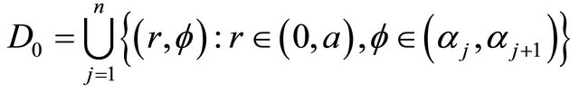 or
or 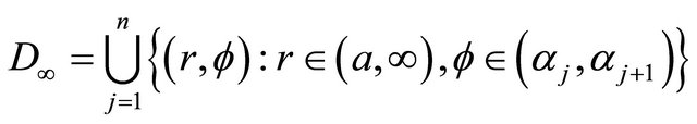 . Here
  denote certain angles such that
 . It is known that if
  satisfies homogeneous boundary conditions on all boundary lines
  in addition to non-homogeneous ones on the circular boundary
![]() , then an explicit expression of
, then an explicit expression of  in terms of eigen-functions can be found through the classical method of separation of variables. But when the boundary condition given on the circular boundary
 ![]() is homogeneous, it is not possible to define a discrete set of eigen-functions. In this paper one shows that if the homogeneous condition in question is of the Dirichlet (or Neumann) type, then the logarithmic sine transform (or logarithmic cosine transform) defined by
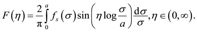
is homogeneous, it is not possible to define a discrete set of eigen-functions. In this paper one shows that if the homogeneous condition in question is of the Dirichlet (or Neumann) type, then the logarithmic sine transform (or logarithmic cosine transform) defined by  (or
(or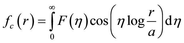 ) may be effective in solving the problem. The inverses of these transformations are expressed through the same kernels on
  or
or . Some properties of these transforms are also given in four theorems. An illustrative example, connected with the heat transfer in a two-part wedge domain, shows their effectiveness in getting exact solution. In the example in question the lateral boundaries are assumed to be non-conducting, which are expressed through Neumann type boundary conditions. The application of the method gives also the necessary condition for the solvability of the problem (the already known existence condition!). This kind of problems arise in various domain of applications such as electrostatics, magneto-statics, hydrostatics, heat transfer, mass transfer, acoustics, elasticity, etc.
1. Introduction
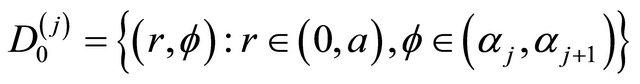
Boundary-value problems connected with sectionallyharmonic functions in wedge-shaped domains

and
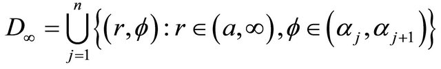 where
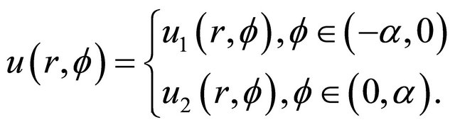
where  stand for the polar coordinates in R2 while a > 0 is a given constant, are important from both pure scientific and engineering points of view. Figure 1 epitomizes a simple case of D0 which corresponds to n = 2. The sub-regions determined by
  and
and  model the regions filled with different materials having different constitutive parameters. The field function
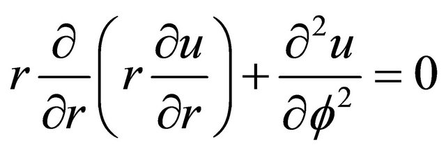
  satisfies the basic equation
 (1a)
(1a)
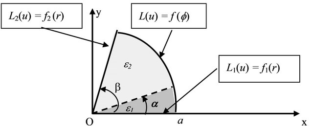
Figure 1. A composite region D0 filled with two different materials.
in the sense of distribution under the boundary conditions
and
shown on the figure. Here  stands for the density of the exciting sources concentrated on the interface
  (if any) while
  and
and  are given linear (differential) boundary operations. The boundary conditions in question may also involve certain terms representing the sources localized on the boundary (if any). As to the function
 , it has constant values e1 and e2 in the sub-regions in question. Thus on the interface between the sub-regions two transmission conditions of the following forms are satisfied:
 (1b)
(1b)
 (1c)
(1c)
As is well-known, when , one can define a set of orthogonal eigen-functions which permit us to obtain an explicit expression of
  in terms of these eigen-functions. The coefficients in the eigen-function series are determined by using the nonhomogeneous boundary condition given on the boundary r = a (i.e. through
 ) together with the regularity condition to be stated at r = 0. When
 , at least one of the functions
  and
and  must be different from zero in order to have a non trivial solution
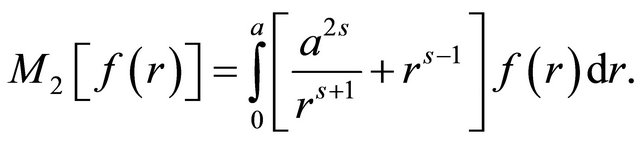
 . In this case it is not possible to define a set of discrete eigen-functions. To overcome such kind of a difficulty, in the midst of the last century some methods, which are effective when the region consists of D0, were proposed. Among them we can mention, for example, the finite Sturm-Liouville transforms introduced by Eringen [1] and Churchill [2], and the finite Mellin transform introduced by Naylor [3,4] (see also [5]). The finite Sturm-Liouville transforms are not appropriate in the case considered here because they are based on the set of eigen-functions which can not be defined in the present case. As to the finite Mellin transforms, they are defined as follows (see, for ex., [5, pp. 462-467]):
 (2a)
(2a)
 (2b)
(2b)
One can easily check that the first or the second transform is appropriate to reduce the Laplace equation written in the circular polar coordinates to an ordinary differential equation when Dirichlet or Neumann type conditions are prescribed, respectively, on the circular part r = a of the boundary. The inverse transforms consist then of the classical Mellin type integrals.
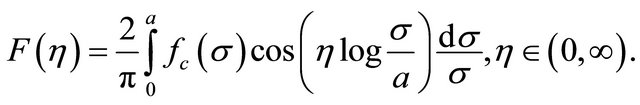
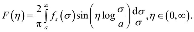
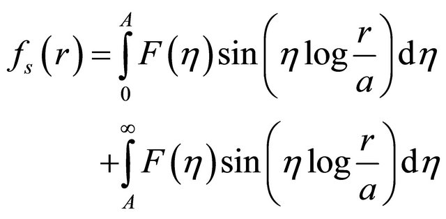
The aim of this note is to show that the transforms of the forms
 (3a)
(3a)
and
 (3b)
(3b)
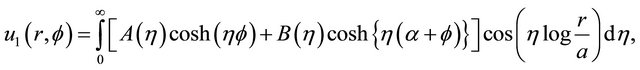
are effective in getting explicit expressions to the solutions of the problems connected with sectionally-harmonic functions defined in D0 and D¥ mentioned above when the boundary condition on the arc r = a is homogeneous and of the Dirichlet or Neumann type. The simplicity of these transforms is that their inverses are also given with the same kernel (see Section 2B below). To clarify the essential properties of the representations ((3a), (b)), in what follows we will consider, without loss of generality, the case where n = 1 (see Figures 2 and 3).
To the best of our knowledge a representation of the form (3b) was first considered by Smythe (see [6, pp. 71-72]) to find the electrostatic potential due to a line source located parallel to a dielectric wedge for which . His discussion is based on moot physical arguments and some particular restrictions. As we will show later on, a representation of the form (3b) is not suitable when
  because only the data known for
  or
or  is sufficient to uniquely
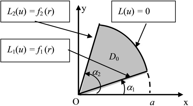
Figure 2. A wedge-shaped region involving only the singular point r = 0.
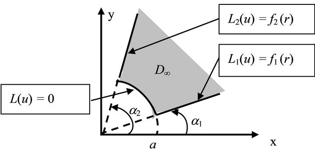
Figure 3. A wedge-shaped region involving only the singular point r = ¥.
determine  (i.e. the inverse transform). Furthermore, when (3b) is used to express
  for all
 , it gives
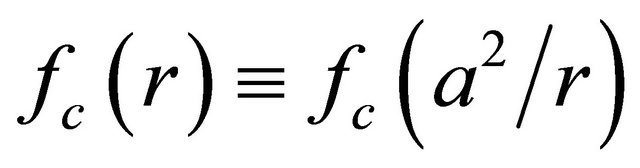 , which is not acceptable from physics point of view.
2. Logarithmic Sine and Cosine Transforms
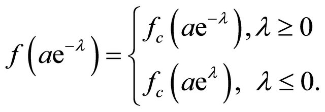
Let a > 0 be a given constant while  is a given function. Then consider the functions
  and
and  defined through the convergent integrals taking place in (3a) and (3b). There log stands for the principal branch of the logarithm function. We will refer
  and
and  to as the logarithmic sine transform and logarithmic cosine transform of
 , respectively. In what follows we will also denote them by the symbols
  and
and . Some interesting and important properties of these transforms are stated in the theorems given below.
A) Limit Values for r ( 0, r ( a and r ( (
As we will see later on (see Section 2B), the expression of the function  (or
(or ) known only in the interval
  or
or  is sufficient to determine the function
  uniquely. The functions
  and
and  may be piece-wise continuous in these intervals. That means that the limit values of the integrals taking place in (3a) and (3b) as r tends to the end point
  may be different from the values obtained by replacing directly
  in those integrals. From application point of view it is the limiting values that are important. Therefore these limit values must be discussed carefully. The two theorems that follow concern this point (for their proof see Appendix).
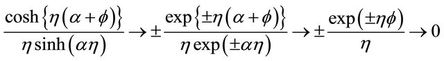
Theorem-1. If , then from (3a) one gets
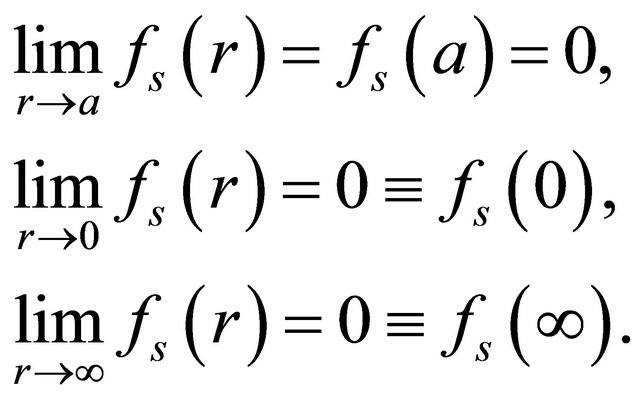 (4a)
(4a)
Theorem-2. a) If , then from (3b) one gets
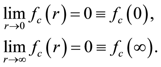 (4b)
(4b)
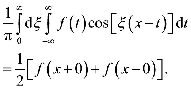
b) If one has also , then
![]() (4c)
(4c)
B) Inverse Transforms
It is an interesting fact that when  (or
(or ) is known for all
  or for all
 , then the function
  can be determined completely. The theorems that follow concern this inversion problem (for their proof see Appendix). Notice that when
  is piece-wise continuous, in what follows
  means
means 
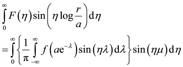
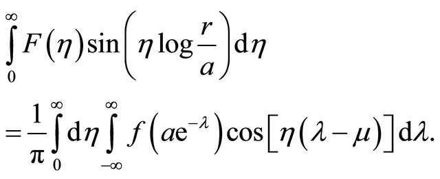
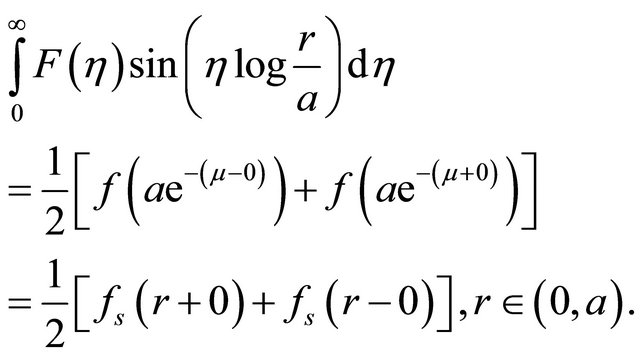
Theorem-3. a) Let  be piece-wise continuous in the interval
  and
and  Then (3a) yields
 (5a)
(5a)
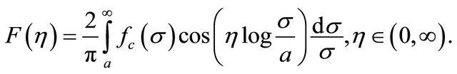
b) If  is piece-wise continuous in the interval
 , then (3b) yields
 (5b)
(5b)
Theorem-4. a) Let  be piece-wise continuous for
  and
and . Then (3a) yields
 (6a)
(6a)
b) If  is piece-wise continuous for
 , then from (3b) one gets
 (6b)
(6b)
The proof of these theorems (except Theorem 1) can easily be achieved by using the already known ones through simple transformations (See for example [5] or [7]). For the sake of fluency of the paper, we prefer to postpone the proofs to the Appendix. In what follows we will denote the inverse transforms given by (5a) and (6a) by . Similarly, the inverse transforms given by (5b) and (6b) will be denoted by
 .
.
3. Applications to Boundary-Value Problems Connected with Sectionally-Harmonic Functions
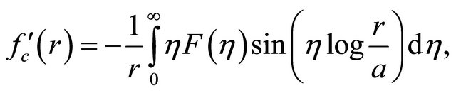
When one has also , by successive differentiations of (3a) and (3b) one gets
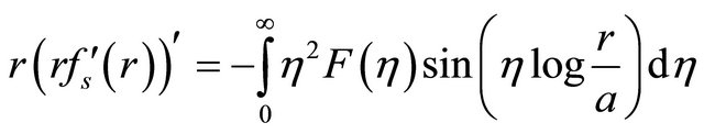 (7a)
(7a)
and
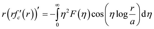 , (7b)
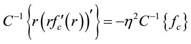
which show that
 (8a)
(8a)
and
 . (8b)
Now consider a function  which is harmonic in
or
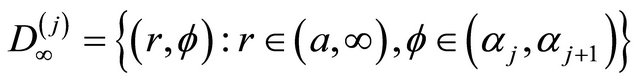
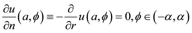
and satisfies a homogeneous boundary condition of the Dirichlet or Neumann type on the circular part of the boundary, namely:
 (9)
(9)
and
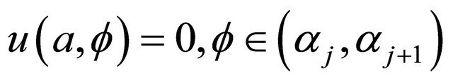 (10a)
(10a)
or
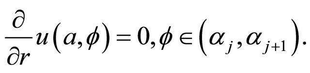 (10b)
(10b)
Application of the operator  or
or  to (9) yields
 (11)
(11)
((8a), (b)) being taken into account. Here  stands for the logarithmic sine or cosine transform of
 . From (11) one gets
 (12)
(12)
where  and
and  are the integration constants to be determined through the boundary and transmission conditions while
  and
and  are two constants which can be chosen appropriately to facilitate the computation. They may also be dependent on h. Thus, in the sector
 one has the following expressions
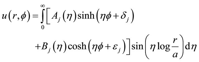 (13a)
(13a)
or
 . (13b)
(13a) is valid for the condition (10a) while (13b) is valid for the case of (10b).
4. An Illustrative Application
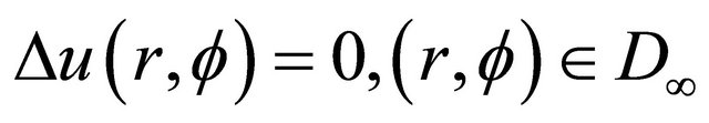
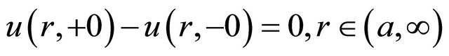
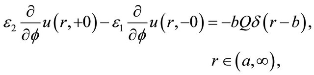
To show the effectiveness of the representations ((13a), (b)), in what follows we will give an illustrative example which concerns the heat conduction in a two-part composite region shown in Figure 4. A point source of amount Q exists at the point (b, 0) while the circular part of the boundary is coated by an insulating material. The physical properties of the lateral boundaries (i.e. the boundary conditions on  and
and ) will be defined later on. Thus the field function (temperature)
  satisfies the following field equation under the given boundary conditions:
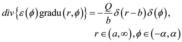 (14)
(14)
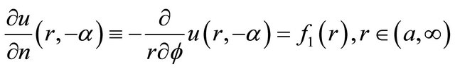 (15a)
(15a)
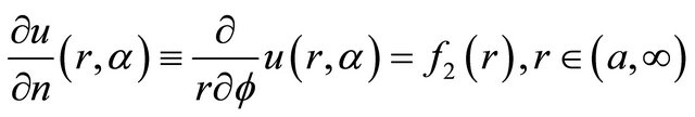 (15b)
(15b)
 (15c)
(15c)
 (15d)
(15d)
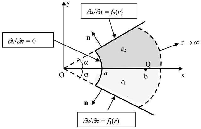
Figure 4. A wedge-shaped region with Neumann type boundary conditions.
Here  has constant values e1 and e2 in the indicated sub-regions.
Remark that the problem posed by (14)-(15d) has a solution if the following necessary condition is satisfied by the boundary conditions :
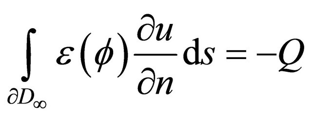 (16a)
(16a)
or, more explicitly,
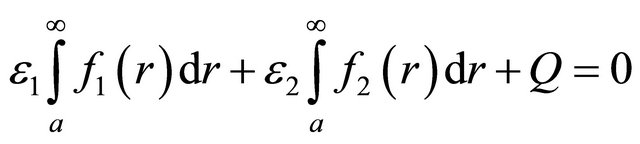 (16b)
(16b)
This is obtained by first integrating (14) on  and then applying the Green’s theorem. In what follows we will assume that (16b) is satisfied (it will be used later on!).
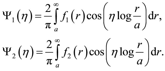
In accordance with the definitions of  and
and let us write
 (17)
(17)
Since the field Equation (14) is equivalent to the equations
 (18a)
(18a)
 (18b)
(18b)
and
 (18c)
(18c)
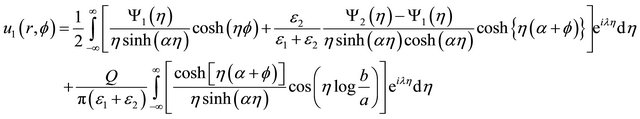
one can write
 (19a)
(19a)
 (19b)
(19b)
The coefficients  and
and  are determined through the conditions (15a), (15b), (18b) and (18c) as follows:
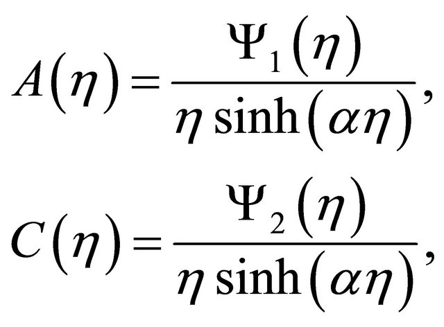 (20a)
(20a)
 (20b)
(20b)
 (20c)
(20c)
Here we put
 (21)
(21)
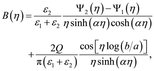
If we first insert (20a)-(20c) into ((19a), (19b)) and then use the Euler formula to write the cos function through exponential functions, then we get
 (22a)
(22a)
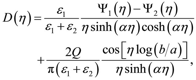
and
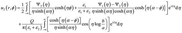 (22b)
(22b)
where l is defined with
 (22c)
(22c)
Now it is important to observe that the point , which is located on the integration line, seems to be a double pole of the integrands in (22a) and (22b). But because of the relation (16b) these poles are removable. Indeed, the removability of these poles requires the condition
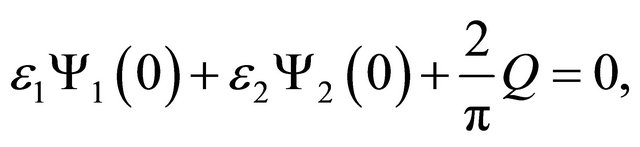 (23)
(23)
which is equivalent to (16b), (21) being taken into account. Since the expressions taking place in the brackets in (22a) and (22b) are even functions of h, (23) guarantees the removability of the singularity at h = 0. Thus, on the basis of Jordan’s lemma, the integrals in ((22a), (b)) can be computed through the residues at the poles located in the upper  or lower
  half-planes. The residue series coming from the poles which occur at the zeros of sinh(ah) and cosh(ah) are connected with the geometry of the wedge in question and, hence, consist of the eigen-functions series. But the terms coming from the poles of
  and
and  (if any!) are independent of the geometry of the wedge and have no connection with the eigen-functions.
Remark. It is worthwhile to notice here that the convergence of the inverse transform integrals in (22a) and (22b) requires the relation (23). That means that the relation stated by (23) is in fact a condition for the existence of the solution. One can easily check that this is nothing but (16b) (or (16a)). This shows that the application of the transformation in question does not only permit us to obtain an explicit expression of the solution but rather shows also the necessary conditions for the existence of a solution.
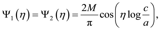
4.1. A Particular Case. Point Sinks Located on the Lateral Boundaries
Assume more particularly that
 (24a)
(24a)
where  and M stand for two given constants such that (Cf. (23) or (16b))
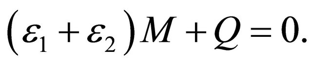 (24b)
(24b)
In this case the lateral boundaries consist of insulating materials and carry sinks at the points  and
and . By straightforward computations one gets
 (24c)
(24c)
which reduces (22a) to
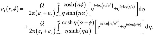 (25)
(25)
Since in the present case one always has
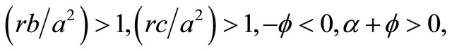
which yields
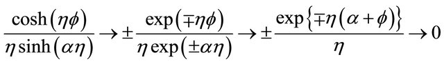 as
as 
 as
as by the Jordan’s lemma, the first parts of these integrals can be computed by considering the residues of the poles taking place in the upper half-plane
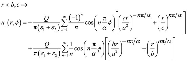
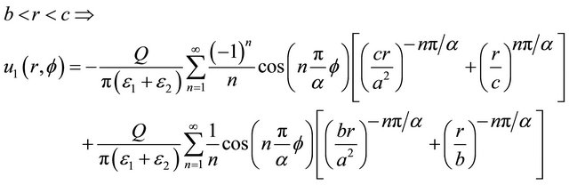
 . But, depending on the relative positions of r and c, one can get
  or
or . Therefore the second part of the first integral involves the contributions of the poles existing in the half-plane
  or
or  (similar situation is also valid for the second part of the second integral). Thus, we have to consider the following four cases separately:
Case 1:  case 2:
Case 3:  case 4:
By straightforward computations we get the following results:
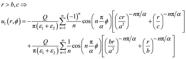 (26a)
(26a)
 (26b)
(26b)
 (26c)
(26c)
 (26d)
(26d)
By comparing (22b) with (22a) one observes that , where
 . It is also interesting to compare (26a)-(26d) with the result pertinent to the case of
 . Thus one concludes that the present two-part wedge problem is equivalent to the homogeneous wedge problem with constitutive parameter
  .
.
5. Conclusions and Concluding Remarks
From the analysis made above one concludes that the logarithmic transformations defined by (3a) and (3b) may be appropriate in getting explicit expressions of sectionally-harmonic functions which satisfy the homogeneous Dirichlet or Neumann boundary conditions on the circular part of the boundary of wedge shaped domains. This kind of problems arise in various domain of applications such as electrostatics, magneto-statics, hydrostatics, heat transfer, mass transfer, acoustics, elasticity, etc.
REFERENCES
- A. C. Eringen, “The Finite Sturm-Liouville Transform,” Quarterly Journal of Mathematics, Vol. 5, No. 1, 1954, pp. 120-129. doi:10.1093/qmath/5.1.120
- R. V. Churchill, “Generalized Finite Fourier Cosine Transforms,” Michigan Mathematical Journal, Vol. 3, No. 1, 1955, pp. 85-94. doi:10.1307/mmj/1031710540
- D. Naylor, “On a Mellin Type Integral Transform,” Journal of Mathematics and Mechanics, Vol. 12, No. 2, 1963, pp. 265-274.
- D. Naylor, “On an Integral Transform of the Mellin Type,” Journal of Engineering Mathematics, Vol. 14, No. 2, 1980, pp. 93-99. doi:10.1007/BF00037619
- I. N. Sneddon, “The Use of Integral Transforms,” McGrawHill Co., New York, 1972.
- W. R. Smythe, “Static and Dynamic Electricity,” McGrawHill Co., New York, 1950.
- E. C. Titchmarsh, “An Introduction to the Theory of Fourier Integrals,” Oxford University Press, 1948.
Appendix. Proof of Theorems
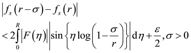
1. A Proof for Theorem-1
 is quite obvious. To find the limit of
  for
for![]() , consider first the case when
, consider first the case when  and assume that an arbitrarily fixed (small)
  is given. Since
 , we can find an
  such that
 (27a)
(27a)
Thus, from (3a) one gets
which yields
 (27b)
(27b)
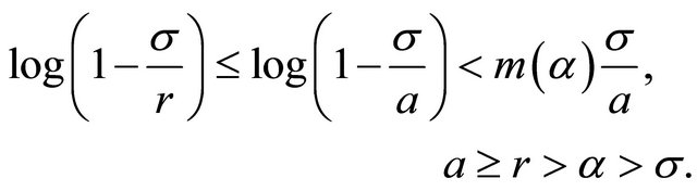
Now, by taking into account the inequalities (see Figure A1).
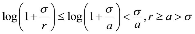 (27c)
(27c)
and
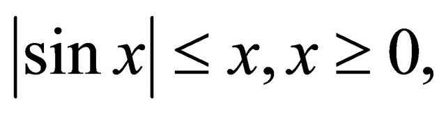
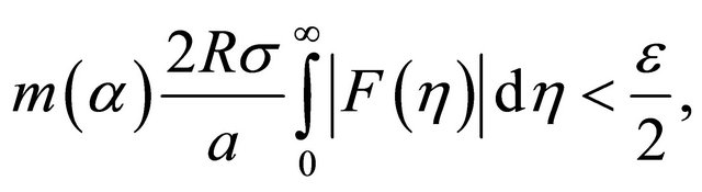
we can choose s so small that
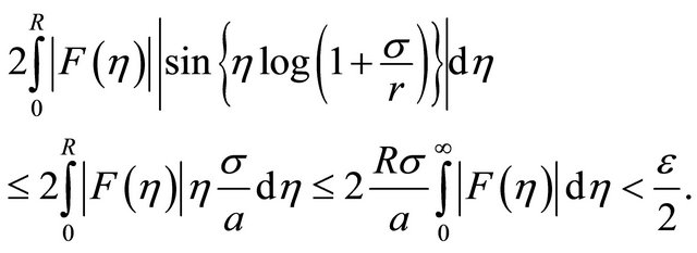 (27d)
(27d)
From (27b) and (27d) we conclude that for every , however it is small, we can find
  such that
which permits us to write
For ![]() this gives the first equation in (4a).
this gives the first equation in (4a).
To prove the same equality for the case of , we choose an arbitrary number
  and repeat the arguments made above by replacing
 ![]() by
by . All the lines except (27b) and (27c) remain unchanged while the latter become now as follows:
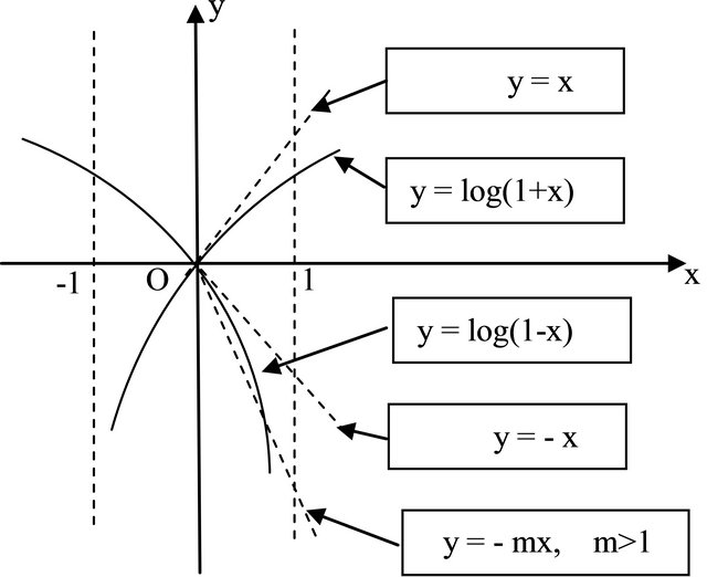
Figure A1. Logarithm functions.
 (28a)
(28a)
and
 (28b)
(28b)
Here  stands for a suitable number which does not depend on s (For detail see Figure A1). Thus, by choosing s sufficiently small, we guarantee
 (28c)
(28c)
which yields
and
 (28d)
(28d)
For r = a the latter reduces to the first equality in (4a) when 
To see the limit of  as r®0, consider an arbitrarily given (small)
  and choose
  such that the second part in
 (29a)
(29a)
meets the following inequality:
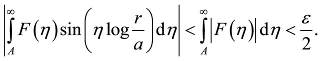 (29b)
(29b)
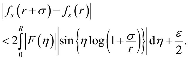
After having fixed A, let us make . By virtue of the well-known Riemann-Lebesgue lemma [5, p. 30], the first part in (29a) tends to zero when
 . Therefore, for sufficiently small r one has also
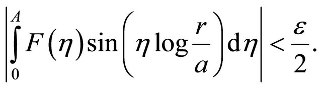 (29c)
(29c)
From (29a)-(29c) one concludes that for sufficiently small r one has  for every
  This proves the second equality in (4a).
(29a)-(29c) are also valid for r ® ¥, which shows the last equality in (4a)
2. A Proof for Theorem-2
The equalities given in (4b) can be shown by repeating the reasoning made in proving Theorem-1. As to the equality given in (4c), owing to the assumption

and
 (30)
(30)
it is reduced to the first equality in (4a).
3. Proofs of Theorem-3 and 4
Proof of these theorems are based on the following wellknown lemma (see [5, p. 34]).
Lemma (Fourier’s integral theorem). If  is piece-wise continuous and absolutely integrable in
 , then for all
  one has
 (31)
(31)
Let us insert (5a) into the right-hand side of (3a) and make the substitutions
 (32a)
(32a)
which yield
 (32b)
(32b)
and
 (33a)
(33a)
Now let us define the odd function
as follows (notice that ):
):
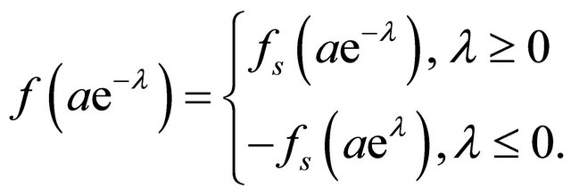 (33b)
(33b)
Then (33a) can also be written as
 (33c)
(33c)
or
 (33d)
(33d)
Since the function  meets the requirements mentioned in the lemma, from the last expression one gets
 (34)
(34)
This proves (5a).
To prove (5b), one starts from (3b) and repeats (32a)- (34) with the only exception that (33b) is replaced now by the even function
Proof of theorem-4 is quite similar to that of Theorem-3. The only difference is that l and m defined in (32a) are replaced now by
and
 .
.