Applied Mathematics
Vol. 3 No. 11 (2012) , Article ID: 24520 , 5 pages DOI:10.4236/am.2012.311235
A Note on the Proof of the Perron-Frobenius Theorem
1University of Chicago, Chicago, USA
2University of Texas, Austin, USA
3Texas A&M University—Qatar, Doha, Qatar
Email: yc9z@uchicago.edu, tcarson@math.utexas.edu, mohamed.elgindi@qatar.tamu.edu
Received September 13, 2012; revised October 14, 2012; accepted October 21, 2012
Keywords: Perron Eigenpair; Homotopy; Eigencurves; Positive Matrices; Interval Matrices
ABSTRACT
This paper provides a simple proof for the Perron-Frobenius theorem concerned with positive matrices using a homotopy technique. By analyzing the behaviour of the eigenvalues of a family of positive matrices, we observe that the conclusions of Perron-Frobenius theorem will hold if it holds for the starting matrix of this family. Based on our observations, we develop a simple numerical technique for approximating the Perron’s eigenpair of a given positive matrix. We apply the techniques introduced in the paper to approximate the Perron’s interval eigenvalue of a given positive interval matrix.
1. Introduction
A simple form of Perron-Frobenius theorem states (see [1,2]):
If  is a real
  matrix with strictly positive entries
 , then:
1) A has a positive eigenvalue r which is equal to the spectral radius of A2) r is a simple3) r has a unique positive eigenvector v4) An estimate of r is given by the inequalities:

The general form of Perron-Frobenius theorem involves non-negative irreducible matrices. For simplicity, we confine ourselves in this paper with the case of positive matrices. The proof, for the more general form of the theorem can be obtained by modifying the proof for positive matrices given here.
Perron-Frobenius theorem has many applications in numerous fields, including probability, economics, and demography. Its wide use stems from the fact that eigenvalue problems on these types of matrices frequently arise in many different fields of science and engineering [3]. Reference [3] discusses the applications of the theorem in diverse areas such as steady state behaviour of Markov chains, power control in wireless networks, commodity pricing models in economics, population growth models, and Web search engines.
We became interested in the theorem for its important role in interval matrices. The elements of an interval matrix are intervals of . In [4], the theorem is used to establish conditions for regularity of an interval matrix. (An interval matrix is regular if every point in the interval matrix is invertible). In Section 4 we develop a method for approximation of the Perron’s interval eigenvalue of a given positive interval matrix. See [5] for a broad exposure to interval matrices.
Since after Perron-Frobenius theorem evolved from the work of Perron [1] and Frobenius [2], different proofs have been developed. A popular line starts with the Brouwer fixed point theorem, which is also how our proof begins. Another popular proof is that of Wielandt. He used the Collatz-Wielandt formula to extend and clarify Frobenius’s work. See [6] for some interesting discussion of the different proofs of the theorem.
It is interesting how this theorem can be proved and applied with very different flavours. Most proofs are based on algebraic and analytic techniques. For example, [7] uses Markov’s chain and probability transition matrix. In addition, some interesting geometric proofs are given by several authors: see [8,9]. Some techniques and results, such as Perron projection and bounds for spectral radius, are developed within these proofs. More detailed history of the geometry based proofs of the theorem can be found in [8].
In our proof, a homotopy method is used to construct the eigenpairs of the positive matrix A. Starting with some matrix  with known eigenpairs, we find the eigenpairs of the matrix
  for t starting at 0 and going to 1. If for each t all eigenvalues of
  are simple, then the eigencurves
  do not intersect as t varies from 0 to 1.
Our proof requires that the curve formed by the greatest eigenvalues  and its reflection about the real axis (i.e.,
 ) will not intersect with any other eigencurve. Together they form a “restricting area” for all other eigenvalue curves. As a result, the absolute value of any other eigenvalue will be strictly less than
  for
for . By choosing an initial matrix
  that has the desired properties stated in the Perron-Frobenius theorem, we will show that the “restricting area” preserves these properties along the eigencurves for all
 , and for
  in particular.
Our proof is elementary, and therefore is easier to understand than other proofs. While most of the other proofs focus on the matrix A itself, we approach the problem by analysing a family of matrices. In our proof we study some intuitive structures of the eigenvalues of positive matrices and show how those structures are preserved for matrices in a homotopy. Thus, our proof provides an alternative perspective of studying the behaviour of eigenvalues in a homotopy.
Furthermore, our proof is constructive. The idea is to start with the known eigenpair corresponding to the maximal eigenvalue of , then use the homotopy method and follow the eigencurve corresponding to the maximal eigenvalues of positive matrices
 , applying techniques such as Newton’s method. Recently, many articles are devoted to using homotopy methods to find eigenvalues, for example see [10-12] and the references therein. In most cases, the diagonal of A is used as starting matrix
 . Still, people are interested in finding a more efficient
 , one which has a smaller difference from A. The
  constructed in our proof provides an alternative to the query. It is promising because by proper scaling, it can behave as some “average” matrix.
2. The Proof
In the following sections,  will denote a real
  matrix with strictly positive entries, i.e.
 . If
. If  is an eigenvalue for A, and v is its corresponding eigenvector, then
  forms an eigenpair for A. A vector is positive if all of its components are positive. An eigenpair is positive if both of its eigenvalue and eigenvector components are positive.
Lemma 2.1.  has a positive eigenpair
 .
.
Proof. Define the function  to be:
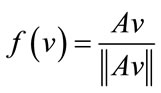
where
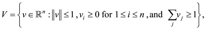
and  denotes the maximum norm of
Then f is continuous (since V does not contain the zero vector and  is positive for any v in V), V is convex and compact (since V is closed and bounded, it is compact, while convexity follows trivially),
  (since the maximum norm of v in V is dominated by
 ). According to Brouwer fixed point theorem, a continuous function f which maps a convex compact subset K of a Euclidean space into itself must have a fixed point in K. Thus, there exists v in V such that
 . No component of v can be 0, since any positive matrix operating on a non-negative vector with at least one positive element will result in a strictly positive vector. So v is a positive eigenvector of A, and the associated eigenvalue r is also positive.
Lemma 2.2. If r is the positive eigenvalue associated with the eigenvector v in the previous lemma, then r has no other (independent) eigenvector.
Proof. Suppose on the contrary, there is another positive eigenvector x for r. Assume that x and v are independent.
Let
Let m be an index such that . Let
. Let , then y is an eigenvector for A associated with eigenvalue r. It’s clear that
  and
and  for all i. Since x and v are linearly independent,
 . Therefore,
 . On the other hand,
  , a contradiction. Therefore v is the only eigenvector for r.
Lemma 2.3. v is the only positive eigenvector for A.
Proof. Suppose on the contrary, there is another positive eigenvector x (independent of v) associated with an eigenvalue . It’s clear that
 . According to Lemma 2.2,
 . Without loss of generality, assume
 . Suppose

Let , then just as in the previous lemma,
  ,
,  for all i, and
 . It follows that
  is a positive vector.
But , which contradicts
  .
.
Remark. The previous lemmas imply that there exists a unique positive eigenpair  for A.
Lemma 2.4. There is no negative eigenvalue  for A such that
 , where
  is the positive eigenpair of A.
Proof. Suppose the statement of the lemma is false. It follows that there exists an eigenpair  such that
 . Then
  is an eigenpair for
 . On the other hand,
  is also an eigenpair for
 . There are two different eigenvectors associated with
 . Since
  is a positive matrix, this contradicts Lemma 2.2 and this completes the proof of this lemma.
Lemma 2.5. Suppose . Then
 ,
,  such that
 (1)
(1)
 (2)
(2)
Proof. Inequalities (1) and (2) are equivalent to
 (3)
(3)
 (4)
(4)
According to Dirichlet’s approximation theorem, for any , there is
  such that
Let .
.
Then  satisfy (3).
Now let . If
. If , then
  satisfy (4). If
 , then
so  satisfy (4).
Lemma 2.6. There does not exist complex eigenvalue  of A such that
 .
.
Proof. Suppose, on the contrary, that there exists an eigenpair  such that
 , where
  and
and . Let
. Let . It’s impossible that
 for all j, for this would make
for all j. However, it’s clear that  when
when .
.
Therefore, there exists some xj such that . (if not, then consider
 ). Suppose
and t is obtained at . Let
. Let , then
  for all i. Either
  or there exists some n such that
 . Since if
  for all i, then let m be the index of the element with non-zero imaginary part. For any
 ,
,
If , then according to lemma 2.5, there exists
  such that
It follows that , a contradiction.
The case for  is similar.
If , then there exists some p such that
 . Let
. Let ,
, . Require
  to be sufficiently small so that
  is still a positive vector. It follows that for any
 ,
,
 . But according to lemma 2.5, for any
 , there exists
  such that
  . Then
 . This again results in a contradiction, and hence the eigenpair
  does not exist.
Remark. The previous lemmas imply that if  is the unique positive eigenpair of
 , then
  is equal to the spectral radius of A (since if
  is any eigenpair corresponding to an eigenvalue of the maximum absolute value, then it can be shown that
  is an eigenpair with positive eigenvector, and the above lemmas will then imply that
 .)
.)
Lemma 2.7. The matrix
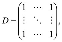
has a simple eigenvalue n and eigenvalue 0 with algebraic multiplicity . In addition, the eigenvector associated with n is positive.
Proof. Since , n is an eigenvalue of D. Likewise,
  are
are  independent eigenvectors of D associated with the eigenvalue 0. So 0 is an eigenvalue for D with multiplicity
 . Since an
  matrix have only n eigenvalues, these are all the eigenvalues of D. Therefore, the eigenvalue of the greatest absolute value of D is positive and simple, and its corresponding eivenvector has positive entries.
Theorem 2.1. Let A be any positive matrix. Then A has a positive simple maximal eigenvalue r such that any other eigenvalue λ satisfies  and a unique positive eigenvector v corresponding to r. In addition, this unique positive eigenpair,
  , can be found by following the maximal eigenpair curve
  of the family of matrices
where D is the  matrix with defined in lemma 2.7.
Proof. The first part of the statement of the theorem follows from the previous lemmas. We will denote the eigenpair of the matrix D by  and
and  .
.
 ,
,  , are all positive matrices. We will now examine the eigencurves
 , where
 is a particular eigenvalue for
 , and
, and  is an eigenvector associated with it. The eigencurve
  starting at
  is not going to intersect any other eigencurve at any time and
  remains to be the largest eigenvalue. Therefore, the unique positive eigenpair,
  of the matrix A, can be found by following the maximal eigenpair curve
 .
.
Theorem 2.2. An estimate of r is given by:

Proof. Suppose
then

Therefore
Remark. This completes the proof of Perron-Frobenius theorem for positive matrices. The proof can be modified to prove the more general case for irreducible non-negative matrices. For example, this can be done by letting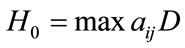 , where D is the matrix defined in Lemma 2.7. As we noted in the introduction, we will next demonstrate how to use homotopy method to find the largest eigenvalue of a positive matrix A numerically.
3. Numerical Example
In this section we use the homotopy method to approximate the positive eigenpair of the matrix:
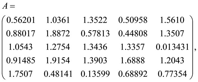
starting with the 5 × 5 matrix D of all entries ones. In [12] it is shown that the homotopy curves that connect the eigenpairs of the starting matrix D and those of A can be followed using Newton’s method. We use these techniques to follow the eigencurve associated with the largest eigenvalue of D. While [12] finds all the eigenvalues of tridiagonal symmetric matrices, the method works well in approximating the largest eigenvalue when it is applied to any positive matrix due to the separation of its eigencurves (see [12] for details).
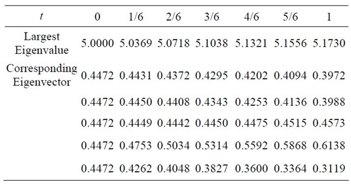
The eigenpath of , shown in Figure 1, is constructed using the numerical results presented in the following table:
4. An Application to Positive Interval Matrices
To differentiate ordinary matrices in the previous sections from interval matrices, we will call them point matrices in this section. As stated in Section 1.2, an interval matrix is of the form , where
  and
and 
are point matrices.
Definition 4.1. We call A a positive interval matrix if  and
and  are positive. The set E is Perron’s interval eigenvalue of A if E consists of all positive real maximal eienvalues of all the positive point matrices B with
 .
.
We are interested in determing Perron’s interval eigenvalue E of A. We’ll show that if s = the Perron’s eigenvalue of , t = the Perron’s eigenvalue of
 , then
 . Therefore, we can approximate E using the Homotopy method introduced in this paper.
Lemma 4.1. Let B be an  positive point matrix with Perron’s eigenpair
 , and C be an
  positive point matrix with Perron’s eigenpair
 . Suppose
  for all
 , then
 .
.
Proof. Let , and suppose the maximum is obtained when
 . Then
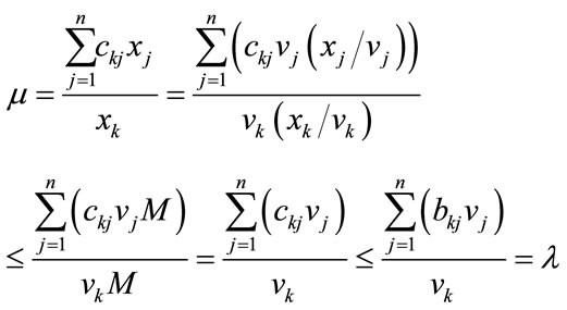
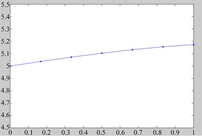
Figure 1. The maximal eigenvalue path for A.
Theorem 4.1. Let  be a positive interval matrix, and E is its Perron’s interval eigenvalue. Suppose
  the Perron’s eigenvalue of
 ,
,  the Perron’s eigenvalue of
 , then
 .
.
Proof. For any  and
and , we have
 . Suppose
  is the Perron’s eigenvalue of B, then
  from the previous lemma. Therefore
 .
.
Let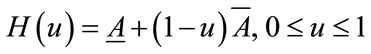 . Define the function
  to be:
Then  and
and . Since f is continuous, then from the Intermediate Value Theorem, for all
  there’s some
  such that
 . Therefore
 .
.
It follows that 
Remark. Theorem 4.1 shows that in order to find the Perron’s interval eigenvalue E of A, we only need to find the Perron’s eigenvalues of  and
and , which can be approximated using the technique introduced in the previous section.
5. Acknowledgements
This research was partially carried out by two students: Yun Cheng and Timothy Carson, under the supervision of Professor M. B. M. Elgindi, and was partially sponsored by the NSF Research Experience for Undergraduates in Mathematics Grant Number: 0552350 and the Office of Research and Sponsored Programs at the University of Wisconsin-Eau Claire, Eau Claire, Wisconsin 54702-4004, USA.
REFERENCES
- O. Perron, “The Theory of Matrices,” Mathematical Annalem, Vol. 64, No. 2, 1907, pp. 248-263.
- G. Frobenius, “About Arrays of Non-negative Elements,” Reimer, Berlin, 1912.
- S. U. Pillai, T. Suel and S. Cha, “The Perron-Frobenius Theorem: Some of Its Applications,” IEEE in Signal Processing Magazine, Vol. 22, No. 2, 2005, pp. 62-75.
- J. Rohn, “Explicit Inverse of an Interval Matrix with Unit Midpoint,” Electronic Journal of Linear Algebra, Vol. 22, 2011, pp. 138-150.
- J. Rohn, “A Handbook of Results on Interval Linear Problems,” 2005. http://uivtx.cs.cas.cz/ rohn/publist/!handbook.pdf
- F. R. Gantmache, “The Theory of Matrices, Volume 2,” AMS Chelsea Publishing, Providence, 2000.
- University of Nebraska-Lincoln, “Proof of Perron-Frobenius Theorem,” 2008. http://www.math.unl.edu/~bdeng1/Teaching/math428/Lecture%20Notes/PFTheorem.pdf
- A. Borobia and U. R. Trfas, “A Geometric Proof of the Perron-Frobenius Theorem,” Revista Matematica de la, Vol. 5, No. 1, 1992, pp. 57-63.
- H. Samelson, “On the Perron-Frobenius Theorem,” The Michigan Mathematical Journal, Vol. 4, No. 1, 1957, pp. 57-59.
- T. Zahng, K. H. Law and G. H. Golub, “On the Homotopy Method for Symmetric Modified Generalized Eigenvalue Problems,” 1996. http://citeseerx.ist.psu.edu/viewdoc/summary?doi=10.1.1.49.7261
- M. T. Chu, “A Note on the Homotopy Method for Linear Algebraic Eigenvalue Problems,” North Carolina State University, Raleigh, 1987.
- P. Brockman, T. Carson, Y. Cheng, T. M. Elgindi, K. Jensen, X. Zhoun and M. B. M. Elgindi, “Homotopy Method for the Eigenvalues of Symmetric Tridiagonal Matrices,” Journal of Computational and Applied Mathematics, Vol. 237, No. 1, 2012, pp. 644-653. doi:10.1016/j.cam.2012.08.010
NOTES
*Sponsored by NSF Grant Number: 0552350.