Applied Mathematics
Vol.3 No.10A(2012), Article ID:24119,8 pages DOI:10.4236/am.2012.330194
A Parallel Algorithm for Global Optimization Problems in a Distribuited Computing Environment
Department of Mathematics and Informatics, University of Cagliari, Cagliari, Italy
Email: gaviano@unica.it, lera@unica.it, elisabetta.mereu@hotmail.it
Received July 4, 2012; revised August 4, 2012; accepted August 11, 2012
Keywords: Random Search; Global Optimization; Parallel Computing
ABSTRACT
The problem of finding a global minimum of a real function on a set S  Rn occurs in many real world problems. Since its computational complexity is exponential, its solution can be a very expensive computational task. In this paper, we introduce a parallel algorithm that exploits the latest computers in the market equipped with more than one processor, and used in clusters of computers. The algorithm belongs to the improvement of local minima algorithm family, and carries on local minimum searches iteratively but trying not to find an already found local optimizer. Numerical experiments have been carried out on two computers equipped with four and six processors; fourteen configurations of the computing resources have been investigated. To evaluate the algorithm performances the speedup and the efficiency are reported for each configuration.
1. Introduction
In this paper we consider the following global optimization problem.
Problem 1

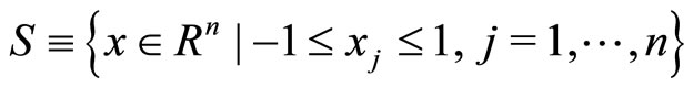
where f: S→R is a function defined on a set S  Rn .
Rn .
In order to solve Problem 1 a very large variety of algorithms has been proposed; several books that describe the research trends from different points of view, have appeared in the literature [1-8]. Numerical techniques for finding solutions to such problems by using parallel schemes have been discussed in the literature (see, e.g. [9-13]. To generalize the investigation of the properties of the algorithms, these are classified in families whose components share common strategies or techniques. In [14] five basic families are defined: partition and search, approximation and search, global decrease, improvement of local minima, enumeration of local minima. Nemirovsky and Yudin [15], and Vavasis [16] have proved, under suitable assumptions, that the computational complexity of the global optimization problem is exponential; hence, the number of function evaluations required to solve problem 1 grows dramatically as the number of variables of the problem increases. This feature makes the search of a global minimum of a given function a very expensive computational task. On the other hand the latest computers in the market, equipped with more than one processor, and clusters of computers can be exploited. In [17] a sequential algorithm, called Glob was presented; this belongs to the improvement local minima family and carries on local search procedures. Specifically, a local minimum finder algorithm is run iteratively and in order to avoid to find the same local minimizer, a local search execution rule was introduced; this was chosen such that the average number of function evaluations needed to move from a local minimum to a new one, is minimal. The parameters used to define the execution rule at a given iteration were computed taking into account the previous history of the minimization process.
In this paper we present a parallel algorithm that distributes the computations carried out by Glob across two or more processors. To reduce to a low level the data passing operations between processors, the sequential algorithm is run on each processor, but the parameters of the execution rule are updated either after a fixed number of iterations are completed or straight as soon as new local minimizer is found. The new algorithm has been tested for solving several test functions commonly used in the literature. The numerical experiments have been carried out on two computers equipped with four and six processors; fourteen configurations of the computing resources have been investigated. To evaluate the algorithm performances the speedup and the efficiency are reported for each configuration.
2. Preliminaries
In this section we recall some results established in [17]. For Problem 1 we consider the following assumption.
Assumption 1
1)  has m local minimum points
  and
and ;
;
2) meas (S) = 1, with meas (S) denoting the measure of S.
Consider the following algorithm scheme.
Algorithm 1 (Algorithm Glob)
Choose  uniformly on S;


repeat
choose x0 uniformly on S;
if
 or
or 
if 
end if
end if
until a stop rule is met;
end
The function rand (1) denotes a generator of random numbers in the interval . Further, we denote by local_search (xo) any procedure that starting from a point
  returns both a local minimum
  of problem 1 and its function value.
In algorithm Glob a sequence of local searches is carried out. Once a local search has been completed and a new local minimum lj is found, a point x0 at random uniformly on S is chosen. Whenever f(x0) is less than f (lj) a new search is performed from x0; otherwise a local search is performed with probability di.
We assume that Problem 1 satisfies all the conditions required to make the procedure local_search (x0) convergent. We have the following proposition.
Proposition 1. Let assumption 1 hold and consider a run of algorithm Glob. Then the probability that  is a global minimum of problem 1 tends to one as
 .
.
First, we settle the following notation.
Definition 1
·  starting from x,
  returns local minimum
 ;
;
·  ; starting from x,
  returns local minimum
 ;
;
·  ;
;
·  .
.
We have

We consider the following definitions for algorithm Glob.
Definition 2
·  the probability that having found the local minimum
 , in a subsequent iteration no new local minimum is detected;
· 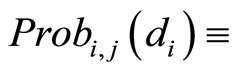 the probability that the algorithm, having found the local minimum
 , can find the local minimum
  in a subsequent iteration.
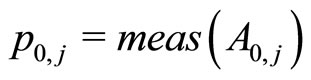
We calculate the average number of function evaluations so that algorithm Glob having found a local minimum, finds any new one. We assume that algorithm Glob can run an infinite number of iterations. Further it is assumed that the values p0,j and pi,j, i = 1, ···, m − 1 and j = 1, ···, m, are known and that the number of function evaluations required by local_search is  constant.
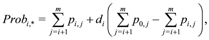
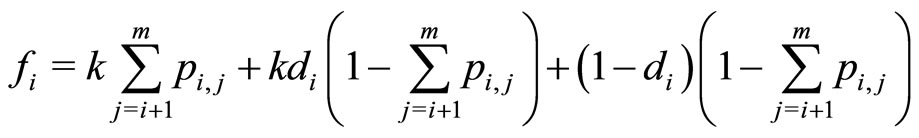
The following holds.
Theorem 1. The average number of function evaluations so that algorithm Glob, having found a local minimum , finds any new one is given by

with
Problem 2. Let us consider problem 1 and let the values k,  and
and  be given. Find value
  such that

We calculate which value of  gives the minimum of such a function. We have as

The derivative sign of  is greater than or equal to zero for
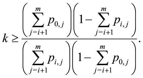 (1)
(1)
The condition (1) links the probability pi,j with the number k of function evaluations performed at each local search in order to choose the most convenient value of di: if the condition is met, we must take di = 0 otherwise di = 1.
In real problems usually we don’t know the values p0,j and pi,j; hence the choice of probabilities d1, d2, ···, dm in the optimization of the function in problem 2 cannot be calculated exactly. By making the following approximation of the values
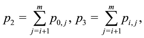
which appear in the definition of evals1 in problem 2, we can device a rule for choosing the values di, I = 1, ···, m in algorithm Glob. Specifically, from (1) we get
where ,
,  and k are approximated as follows
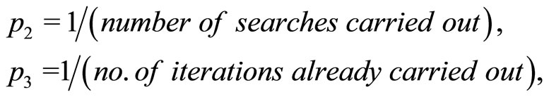 (2)
(2)

Hence the line

of algorithm Glob is replaced by the line
 (3)
(3)
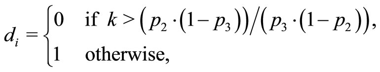
where yes_box ( ) is a procedure that returns zero or 1 and is defined by
Procedure 1 (yes-box())


 ;
;
if 
 ;
;
end if
if 
ratio = ;
;
else
ratio = inf;
end if
if k > ratio yes = 0;
else
yes = 1;
end if
end.
In the sequel we shall denote by Globnew algorithm Glob completed with procedure 1.
3. The Parallel Algorithm
The message passing model will be used in the design of the algorithm we are going to introduce. This model is suitable for running computations on MIMD computers for which according to the classification of parallel systems due to Michael J. Flynn each processor operates under the control of an instruction stream issued by its control unit. The main point in this model is the communication where messages are sent from a sender to one or more recipients. To each send operation there must correspond a receive operation. Further the sender either will not continue until the receiver has received the message or will continue without waiting for the receiver to be ready.
In order to design our parallel algorithm in an environment of N processors we separate functions in two parts: server and client. The server task will executed by just one processor, while the remaining ones will execute the same code. The server will accomplish the following task.
· reads all the initial data and sends them to each client;
· receives the intermediate data from a sender client;
· combines them with all the data already received;
· sends back the updated data to the client sender;
· gathers the final data from each client.
Each client accomplishes the following tasks
· receives initial data from server;
· runs algorithm Globnew;
· sends intermediate data to server;
· receives updated values from server;
· stops running Globnew whenever its stop rule is met in any client execution;
· sends final data to server.
The communication that takes place between the server and each client concerns mainly the parameters in (2), that is, p2, p3 and k. Each client, as soon as he either finds a new local minimizer or a fixed number of iterations have been executed, sends a message to the server containing data gathered after the last sent message; that is.
· last minimum found;
· the number of function evaluations since last message sending;
· the number of iterations since last message sending;
· the number of local searches carried out since last message sending;
· status variable of value 0 or 1 denoting that the stop rule has been met.
The server combines each set of intermediate data received with the ones stored in its memory and sends to the client the new data. If the server receives as status variable 1 in the subsequent messages sent to clients the status variable will keep the same value, meaning that the client has to stop running Globnew and has to send the final data to the server. The initial data and intermediate data are embodied in the following data structures.
· Data_start = struct (“x”, [ ], “fx”, [ ], “sum_ev”, [ ], “sum_tr”, [ ], “sum_ls”, [ ], “fun”, [ ], “call_interval”, [ ]).
· Data_mid = struct (“stop_flag”, [ ], “client”,[ ], “x”, [ ], “fx”, [ ], “sum_ev”, [ ], “sum_tr” [ ], “sum_ls”, [ ])
where the strings within single quotes denote the names of the members of the structure and [ ] its values.
In Data_start the members “x” and “fx” refer to the algorithm starting point as defined by the user; “sum_ ev”, “sum_tr”, “sum_ls” initialize the number of function evaluations, iterations and local searches. “fun” and “call_interval” denote the problem to solve and the number of iterations to be completed before an intermediate data passing has to take place.
In Data_mid “stop_ flag” and “client” refer to the status variable and to the client sender while the remaining members denote values as in Data_start but if the sender is a client the values refer to values gathered since the last message sending, while if the sender is the server the values concern the overall minimization process.
In the Appendix we report in pseudocode the basic instructions of the procedures to be executed in the server and client processors respectively.
4. Numerical Results
In this section we report the numerical results we got in the implementation of the algorithm outlined in the previous sections. First we describe the paradigm of our experiments.
Four test problems have been solved; to test the performance of our algorithm each problem has been chosen with specific features.
Test problem 1
with

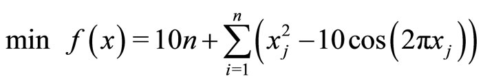
Test problem 2

with

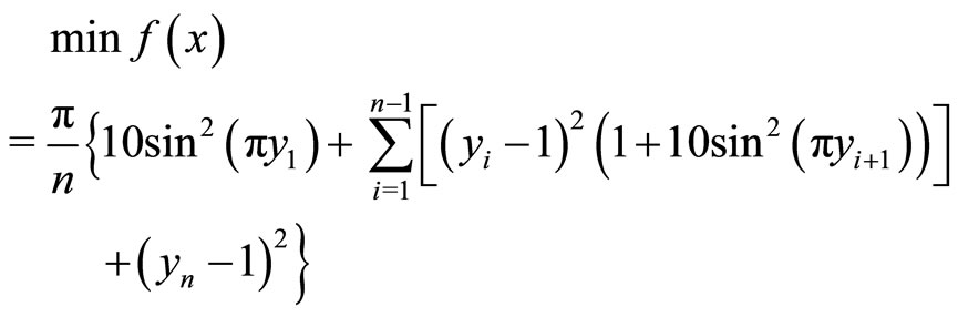
Test problem 3
with

Test problem 4
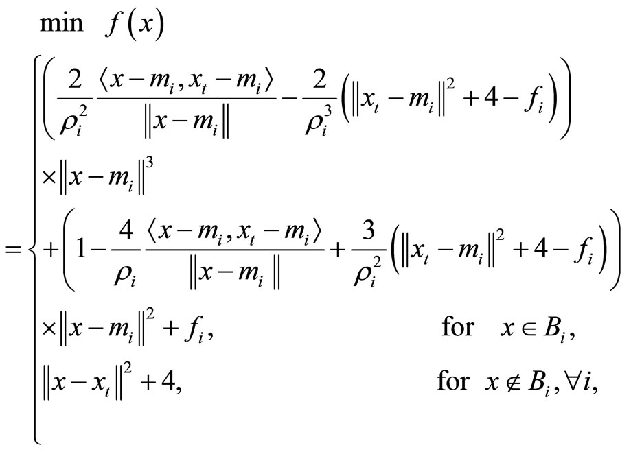
with ,
, 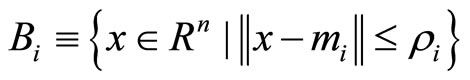 , for
, for  ,
,
 ,
,  , and
, and  denoting ten points uniformly chosen in S such that the
  balls do not overlap each other,
  real values to be taken as the values of
  at
at .
.
Test problems 1, 2, and 3 appeared in [18-20] respectively. Test problems 4 belongs to a set of problems introduced in [21] and implemented in the software GKLS (cfr. [22]).
We have been working in a Linux operating system environment according to the Ubuntu 10.04 LT implementation. All codes have been written in the C language in conjunction with the OpenMPI message passing library (version 1.4.2). The local minimization has been carried out by a code, called cgtrust, written by C. T. Kelley [23]. This code implements a trust region type algorithm that uses a polynomial procedure to compute the step size along a search direction. Since the cgtrust code was written according to the MatLab programming language, this has been converted in the C language. All software used is Open Source.
Two desktop computers have been used; the first equipped with an Intel Quad CPU Q9400 based on four processors, the second with an AMD PHENOM II X6 1090T based on six processors. Experiments have been carried out both on each single computer and on the two connected to a local network. In Table 1 we report the fourteen configurations of the computing resources used in each of our experiments.
Whenever we have being exploiting just one processor of a computer, the running code was written leaving out

Table 1. Configurations of the computing resources.
any reference to the OpenMPI library. Hence the code is largely simpler than the one used for using more than one processor. Since our algorithm makes use of random procedures, to get significant results in solving the test problems, 100 runs of the algorithm have been done on each problem. The data reported in the tables are all mean values. The parameter k that evaluates the computational cost of local searches has been computed as the sum of function and gradient evaluations of the current objective function. The algorithm stops whenever the global minimum has been found within a fixed accuracy. That is the stop rule is

with  and
and  the function values at the global minimum point and at the last local minimum found.
To evaluate the performance of our algorithm we consider two indices, the speedup and the efficiency; the first estimates the decrease of the time of a parallel execution with respect to a sequential run. The second index estimates how much the parallel execution exploit the computer resources. In Tables 2-5 we report the results gathered for each configuration given in Table 1; in each table for each function we report the computational expired time, the speedup and the efficiency. The function evaluation is done in two ways: 1) We evaluate the function as it is defined, 2) We introduce an extra computation that consists of a loop of 5000 iterations where at each iteration the square root of 10.99 is calculated. Hence we carried out our experiments by assigning different weights to the function evaluations. Note that the columns in Tables 4 and 5 referring to one processor has been calculated as the means of the values in the corresponding columns in 2, and 3. From the data in the tables we can state the following remarks.
1) Whenever the function evaluation cost is evaluated
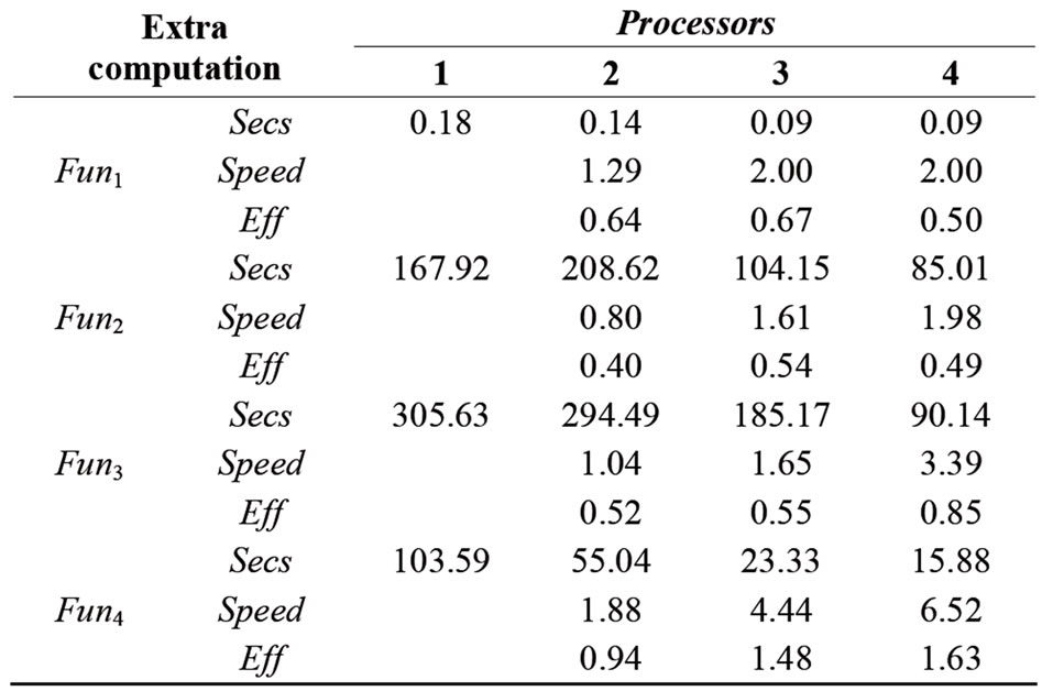
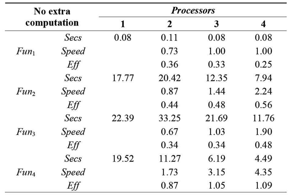
Table 2. Results working with Intel Quad.
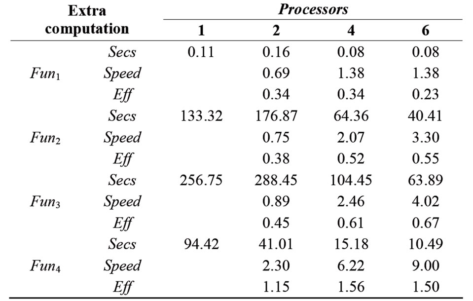
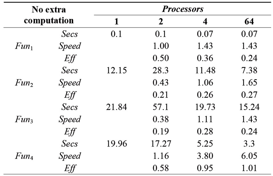
Table 3. Results working with AMD Phenom 6.
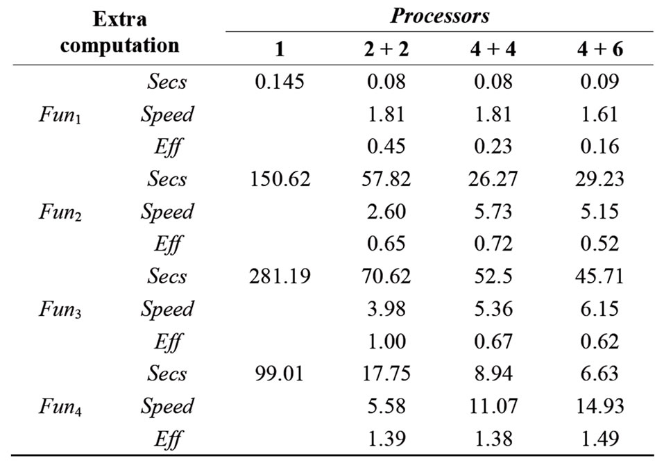

Table 4. Results working with Intel Quad and AMD Phenom 6.
according to
1) The use of more than one processor does not give significant improvements only for the first test problem. Indeed this is a very easy problem to solve and does not require a large computational cost.
2) Working with two processors the speedup becomes less than one. Clearly this has to be related to the fact that the complexity of the multi processor code is not balanced by the use of additional processors.
3) As the function is evaluated according to 2) the advantage of the multiprocessor code becomes clear.
4) The output of the four test problems is quite different; while problem 1 even with the extra computational cost does not exhibits a good efficiency, the remaining problems show significant improvements. For problem 4, the parallel algorithm improves a great deal its performances with respect to the serial version.
5. Conclusion
In order to find the global minimum of a real function of n variables, a new parallel algorithm of the multi-start and local search type is proposed. The algorithm distributes the computations across two or more processors. The data passing between cores is minimal. Numerical

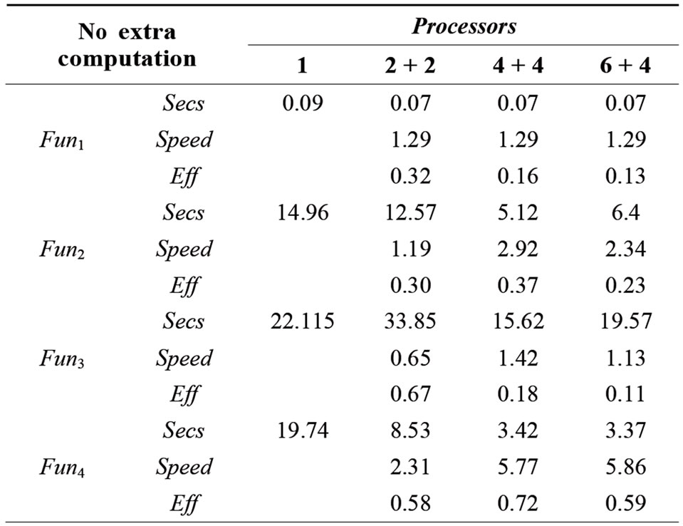
Table 5. Results working with AMD Phenom 6 and Intel Quad.
experiments are carried out in a linux environment and all code has been written in the C language linked to the Open Mpi libraries. Two desktop computers have been used; the first equipped with an Intel Quad CPU Q9400 based on four processors, the second with a AMD Phenom II X6 1090T based on six processors. Numerical experiments for solving four well-known test problems, have been carried out both on each single computer and on the two connected to a local network. Several configurations with up to ten processors have considered; for each configuration, speedup and efficiency are evaluated. The results show that the new algorithm has a good performance especially in the case of problems that require a large amount of computations.
REFERENCES
- R. G. Strongin and Y. D. Sergeyev, “Global Optimization with Non-Convex Constraints. Sequential and Parallel Algorithms,” Kluver Academic Press, Dordrecht, 2000.
- R. Horst and P. M. Pardalos, “Handbook of Global Optimization,” Kluver Academic Press, Dordrecht, 1995.
- R. Horst, P. M. Pardalos and N. V. Thoay, “Introduction to Global Optimization,” Kluver Academic Press, Dordrecht, 1995.
- C. A. Floudas and P. M. Pardalos, “State of the Art in Global Optimization,” Kluwer Academic Publishers, Dordrecht, 1996.
- J. D. Pintér, “Global Optimization in Action,” Kluwer Academic Publishers, Dordrecht, 1996.
- H. Tuy, “Convex Analysis and Global Optimization,” Kluwer Academic Publishers, Dordrecht, 1998.
- P. M. Pardalos and H. E. Romeijn, “Handbook of Global Optimization Volume 2,” Kluwer Academic Publishers, Dordrecht, 2002.
- P. M. Pardalos and T. F. Coleman, “Lectures on Global Optimization,” Fields Communications Series, Vol. 55, American Mathematical Society, 2009, pp. 1-16.
- V. P. Gergel and Y. D. Sergeyev, “Sequential and Parallel Global Optimization Algorithms Using Derivatives,” Computer & Mathematics with Applications, Vol. 37, No. 4-5, 1999, pp. 163-180. doi:10.1016/S0898-1221(99)00067-X
- Y. D. Sergeyev, “Parallel Information Algorithm with Local Tuning for Solving Multidimensional GO Problems,” Journal of Global Optimization, Vol. 15, No. 2, 1999, pp. 157-167. doi:10.1023/A:1008372702319
- E. Eskow and R. B. Schnabel, “Mathematical Modelling of a Parallel Global Optimization Algorithm,” Parallel Computing, Vol. 12, No. 3, 1989, pp. 315-325. doi:10.1016/0167-8191(89)90089-6
- R. Čiegis, M. Baravykaité and R. Belevičius, “Parallel Global Optimization of Foundation Schemes in Civil Engineering,” Applied Parallel Computing. State of the Art in Scientific Computing, Lecture Notes in Computer Science, Vol. 3732, 2006, pp. 305-312.
- G. Rudolph, “Parallel Approaches to Stochastic Global Optimization,” In: W. Joosen and E. Milgrom, Eds., Parallel Computing: From Theory to Sound Practice, IOS, IOS Press, Amsterdam, 1992, pp. 256-267.
- C. G. E. Boender and A. H. G. Rinooy Kan, “Bayesian Stopping Rules for a Class of Stochastic Global Optimization Methods,” Erasmus University Rotterdam, Report 8319/0, 1985.
- A. S. Nemirovsky and D. B. Yudin, “Problem Complexity and Method Efficiency in Optimization,” John Wiley and Sons, Chichester, 1983.
- S. A. Vavasis, “ Complexity issues in global optimization: a survey,” In: R. Horst and P. M. Pardalos, Eds., Handbook of Global Optimization, Kluwer Academic Publishers, Dordrecht, 1995, pp. 27-41.
- M. Gaviano, D. Lera and A. M. Steri, “A Local Search Method for Continuous Global Optimization,” Journal of Global Optimization, Vol. 48, 2010, pp. 73-85.
- A. Levy and A. Montalvo, “The Tunneling Method for Global Optimization,” SIAM Journal on Scientific Computing, Vol. 6, No. 1, 1985, pp. 15-29.
- C. A. Floudas and P. M. Pardalos, “A Collection of Test Problems for Constraint Global Optimization Algorithms,” Springer-Verlag, Berlin Heidelberg, 1990. doi:10.1007/3-540-53032-0
- L. A. Rastrigin, “Systems of Extreme Control,” Nauka, Moscow, 1974.
- M. Gaviano and D. Lera, “Test Functions with Variable Attraction Regions for Global Optimization Problems,” Journal of Global Optimization, Vol. 13, No. 2, 1998, pp. 207-223. doi:10.1023/A:1008225728209
- M. Gaviano, D. E. Kvasov, D. Lera and Y. D. Sergeyev, “Software for Generation of Classes of Test Functions with Known Local and Global Minima for Global Optimization,” ACM, Transaction on Mathematical Software, Vol. 29, No. 4, 2003, pp. 469-480. doi:10.1145/962437.962444
- C. T. Kelley, “Iterative Methods for Optimization,” SIAM, Philadelphia, 1999. doi:10.1137/1.9781611970920
Appendix
Procedure (Glob_server) fun=function to minimize;
np=number of processors;
call_interval=max interval between two server-client messages;
x1=starting point; fx1=fun(x1);
sum_ev=1; sum_tr=0; sum_ls=0;
Data_start=struct(’x’,x1,’fx’,fx1,’sum_ev’,sum_ev’sum_tr’,sum_tr,’sum_ls’,sum_ls,’fun’,fun,’call_ interval’,[ ]).
stop_flag=0;
no_stop=0;
Send Data_start to all clients.
while no_stop<np-1
Receive Data_Mid from any client
sum_ev=sum_ev+Data_mid.sum_ev;
sum_ls=sum_ls+Data_mid.sum_ls;
sum_tr=sum_tr+Data_mid.sum_tr;
if Data_mid.fx>fx1;
Data_mid.x=x1; data_mid.fx=fx1.
else
x1=Data_mid.x; fx1=Data_mid.fx;
end
if Data_mid.stop_flag==1;
no_stops=no_stops+1;
stop_flag=1;
continue
elseif stop_flag==1
Data_mid.stop_flag=1;
no_stops=no_stops+1;
end
send to client Data_mid
end.
Procedure (Glob_client)
client=client_name;
Receive Data_start from server;
x1=Data_start.x; fx1=Data_start.fx;
sum_ls=sum_ls+Data_start.sum_ls;
sum_tr=sum_tr+Data_start.sum_tr;
sum_ev=sum_ev+Data_start.sum_ev;
call_interval=Data_start.call_interval;
buf=struct(’sum_ls’, 0, ’sum_tr’, 0,’sum_ev’, 0);
stop_flag=0;
iter_client=0;
yes=1;
while stop_flag==0
flag_min=0;
iter_client=iter_client+1;
Choose  uniformly on S;
fx=fun(x0);
buf.sum_ev=buf.sum_ev+1;
buf.sum_tr=buf.sum_tr+1;
if fx<fx1 | yes
(x2,fx2,evals)=local_search(x)
buf.sum_ls=buf.sum_ls+1;
buf.sum_ev=buf.sum_ev+evals;
if fx2<fx1
x1=x2; fx1=fx2;
flag_min=1;
end
end
if stop condition satisfied
stop_flag=1;
end
if iter_client==call_interval or flag_min==1 or
stop_flag==1;
Data_mid.stop_flag= stop_flag;
Data_mid.sum_ls=buf.sum_ls;
Data_mid.sum_tr=buf.sum_tr;
Data_mid.sum_ev=buf.sum_ev;
Data_mid.x=x1; Data_mid.fx=fx1;
Data_mid.client=client;
Send Data_mid to server;
Receive Data_mid from server
sum_ls=Data_mid.sum_ls;
sum_tr=Data_mid.sum_tr;
sum_ev=Data_mid.sum_ev;
x1=Data_mid.x;
fx1=Data_mid.fx1;
stop_flag=Data_mid.stop_flag;
buf.sum_ev=0;
buf.sum_tr=0;
buf.sum_ls=0;
iter_client=0;
end
[yes,p2,p3]=yes_box(1,sum_ls,sum_tr,sum_ev
prob_value,iter,itmax);
end.
Send final data to server.