Applied Mathematics
Vol. 3 No. 6 (2012) , Article ID: 20288 , 9 pages DOI:10.4236/am.2012.36093
Black-Scholes Option Pricing Model Modified to Admit a Miniscule Drift Can Reproduce the Volatility Smile
1Financial Guard Ltd., London, UK
2Department of Mathematics and Statistics, Utah State University, Logan, USA
Email: *jim.powell@usu.edu
Received November 2, 2011; revised April 10, 2012; accepted May 17, 2012
Keywords: Option Pricing; Black-Scholes; Volatility Smile
ABSTRACT
This paper develops a closed-form solution to an extended Black-Scholes (EBS) pricing formula which admits an implied drift parameter alongside the standard implied volatility. The market volatility smiles for vanilla call options on the S&P 500 index are recreated fitting the best volatility-drift combination in this new EBS. Using a likelihood ratio test, the implied drift parameter is seen to be quite significant in explaining volatility smiles. The implied drift parameter is sufficiently small to be undetectable via historical pricing analysis, suggesting that drift is best considered as an implied parameter rather than a historically-fit one. An overview of option-pricing models is provided as background.
1. Introduction
An often reiterated view of modern finance states that the Black-Scholes (BS) option pricing formula “accurately reflects” options prices, but this view forgives a free parameter (volatility) which accommodates a considerable degree of variations in option prices. Not only does implied volatility vary over time, but also at any point in time over related options, that is a group of options whose characteristic differ only by strike price. All other characteristic (underlying security, maturity) are identical. This definition does not assume that they use the same volatility for pricing, but it is generally assumed that the same interest rate is applicable. This variation, referred to as the volatility smile or smirk (or sneer), reflects the greater sin, since variation over time could easily be ascribed to changing conditions in the market environment, but variations at any particular instance cannot [1]. This paper addresses these latter variations by offering a slight modification to the BS formula which reflects most of the volatility smile. A (small) drift parameter is added, and a closed-form solution, quite similar to BS, is derived. Using a likelihood ratio test, this new drift parameter is determined to be significant over a sample series of financial data. Furthermore, we argue that this change may explain volatility smiles. To place this model in the proper context, the paper starts with background concerning the volatility smile and the general classes of models used to explain these smiles.
An option is a financial contract between a seller (or writer) and a buyer, in which a buyer, in exchange for a premium, acquires the right (but not the obligation) to buy (for a call option) or sell (for a put option) a specific amount of an underlying commodity at a specified price (the strike price, S) during a specified period of time. This paper focuses on call options. In our notation, w represents the value (or price) of the option at a point in time. At maturity, this value represents the final settlement that the writer pays the seller,  where x is the ending value of the underlying commodity. Only European options are considered, in which there is no possibility of exercise before maturity.
The basic option pricing formula was developed in a series of papers [2-4] (leading to a Nobel Prize for Scholes and Merton in 1997). This model is the Black-Scholes (BS) option pricing formula. Black and Scholes developed a partial differential equation (PDE) relating w (the option price), r (the interest rate), t (time to maturity of the option), x (the price of the underlying security at the current time), and price volatility, v:
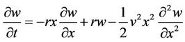 . (1)
. (1)
The volatility, v, is expressed as a fraction of the underlying security (in this paper v is used for volatility rather than the more typically used σ, since the latter will be used to represent model variance from observed prices below). The coefficient of  directly implies a lognormal probability distribution for the price of the underlying security at maturity. Alternatively, Bouchaud and Potters [5] show that the coefficient of the second derivative term in (1) can arise from different assumptions. Initially, the BS option pricing model was viewed to price options without reference to the distribution of the future price of the underlying, except for the free volatility parameter. Currently, it is acknowledged that the option price depends on the assumed or implicit distribution of underlying prices.
Recent research has been motivated, in large part, by the volatility smile (or smirk or sneer) effect, which arises from efforts to explain current prices. Given all the parameters for an option, except volatility, and given a market price for the option, the pricing formula can be inverted to give the implied volatility arising from the market price. If we calculated the implied volatility for a series of options that only differ by strike, we can see how volatility varies with respect to strike. Stereotypical examples are shown in Figure 1. If the profile is symmetric, it is referred to as a “smile”, while asymmetric profiles are “smirks” or “sneers”.
In the original theory, option prices were viewed as a function of the underlying dynamic of the security price changes. It followed that the volatility profile should be a flat line, constant across all strikes, since the considered options only differ by their strike prices; the pricing took place with the same underlying security over the same time to maturity with the same governing interest rates. However, since the stock market crash of 1987, volatility profiles have generally been not flat, rather displaying distinct smiles or smirks, as in Figure 1. That volatility profiles are not flat refutes the basic assumptions of the BS option formula. Recent years have witnessed a flurry
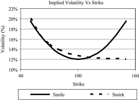
Figure 1. Volatility profiles: Volatility versus strike price. If the profile is symmetric, it is referred to as a “smile”, while asymmetric profiles are “smirks” or “sneers”.
of research to explain the volatility smile, and the focus has been to vary the underlying dynamic of the security prices changes. This process has two goals: to reproduce witnessed option prices and to employ an assumption of security price changes that is reasonable. A number of models have been proposed, outlined below (following Derman [6]).
Local volatility models (or deterministic volatility function models or implied binomial/trinomial tree models) [1,7-9] used current prices to deduce future volatileities. These methods are now out of favor since the implied future volatilities do not exhibit volatility smiles, rather much flatter patterns and lower levels of volatility. Also, the smoothing of local volatility surfaces from discrete option prices constitutes a significant issue.
Stochastic volatility models [10,11] consider both the underlying security and its volatility as stochastic variables. These models reproduce volatility smiles, but initially only symmetric ones. Later, asymmetric prices were reproduced by allowing prices of the underlying security to be correlated with volatility. With these models, hedging (see below) is difficult, primarily because volatility is not an observable statistic, so that a regime shift could not be noted at the time that a hedge transaction would be needed.
More recently innovations have varied aspects of the model other than volatility. Jump diffusion models [3] have been adapted [12] to the stochastic volatility environment by relaxing the continuous assumption of price behavior. Stock modelers, for example, tend to think in downward jumps, like crashes, while energy price modelers might think of price spikes, the latter not only going in the opposite direction but being shorter lived. Appropriate parameters must be incorporated for the frequency, average intensity and standard deviation of intensity, along with any assumptions regarding persistency or mean regression of the new price levels after the jump. These models possess intuitive appeal since dynamics such as crashes, spikes, and perhaps manic periods can be reflected. As a drawback, jump models exaggerate any hedging concerns associated with pure stochastic models; while fast moving markets may be difficult to hedge, jumping ones would seem impossible under in a continuous framework. More recent universal volatility models [13-17] comprise hybrids of the above.
All these models introduce new parameters, for example one or more volatility parameters to create a smile, various distribution parameters for a stochastic volatility model, other parameters to describe jump or other effects. These parameters can be divided into two types: those parameters fitted to historical data and then fixed in the model and those allowed to vary moment to moment as free parameters (similar to implied volatility). The former are called historically-fitted and the latter are implied. Local volatility models generally employ a host of implied volatility parameters and few (if any) historically fitted variables. In contrast, stochastic volatility models employ many historically-fitted parameters and only one implied parameter, the volatility. Jump process parameters are generally historically-fitted.
As discussed above, current research tends to add new parameters to models in an effort to better reflect various aspects of price movements. While doing this, one must be careful that new parameters not only improve the fit but also that the degree of improvement warrants the new parameter. Below we will investigate a one-parameter extension of the BS model which accounts for a small pricing drift. We evaluate its performance compared to the original BS model from the perspective both of reflecting option prices and from that of parsimony: can the increased complexity be justified statistically by the degree of improvement? We fit both the BS and our extension to S&P 500 Options data from 2003-2005; the tradeoff between additional complexity and improved description is assessed using the likelihood ratio test.
2. Mathematical Model and Methods
How would drift come about? There are two alternatives. On the one hand, it may be a small trend that market participants cannot observe. Actual calculations of the drift show it to be quite small, small enough to not be detectable in a statistical analysis of price movements. This view of the drift is consistent with the contention that market dynamics (alone) drive options prices, with negligible distortion by market participants. On the other hand, the drift may be a trend perceived by market participants whether or not it actually exists in the market. This perceived drift alters market prices, but the necessary drift is not small enough to be discredited by statistical analyses. This view is consistent with the contention that market perceptions drive market prices, potentially independent of actual price dynamics. Whichever interpretation appeals to the reader, the mathematics is the same.
It is interesting to note that this additional drift parameter may be viewed as arising from the assumption that the underlying security experiences periods of volatility and periods of relative stagnation. During volatile periods, both random walk effects and interest rates impact option prices. However, during stagnant periods, any pricing effects due to volatility are dormant (by definition) but the interest rate clock would still be running. Thus the implied forward expectation from current option prices would conceptually be composed of two components: one due to the volatility effect (with interest rates during volatile periods), and one due to interest rates (alone) during stagnant periods. The implied drift reflects the difference between interest rate effects and the missing random walk effects over the stagnant periods. The implied drift effect could be positive or negative since the stochastic process during active periods (implied by volatility) could create a forward expectancy above or below that implied by interest rates.
2.1. Deriving an Extension of the Black-Scholes Model
The traditional derivation of BS begins by considering the neutral hedge equity constructed by selling a ratio  of call option in a stock per share of stock held.
Consider the stock and hedging options as a separate portfolio. For such a portfolio the net equity (E) invested is 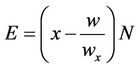 where N is the number of shares of stock held, and subscript notation for partial derivatives is adopted (that is,
 ). Thus
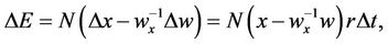
 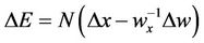 is the net change in portfolio value with changes in either stock or option price. Applying the usual arbitrage-free argument originally introduced by Black, Merton and Scholes, it is required that option prices evolve over time so that equity value experiences growth according to risk-free interest rates. This is natural since the combination of stocks and hedging options constitutes a risk-free portfolio. Mathematically,
 (2)
(2)
where r is the risk-free interest rate. Option price is expected to vary with both time and price of underlying stock; using Taylor’s theorem changes in option price may be replaced with related changes in stock price in time,
 (3)
(3)
The next step would be to substitute (3) into (2) and thereby derive a differential equation for option prices. However, to consistently neglect terms of differing order as , there must be an assumption about how changes in stock price,
  vary with changes in time. As done in the traditional BS assumption, here the assumption is that stock prices follow a random walk process with standard deviation vx in which the market volatility is v. Departing from BS, however, the random walk is assumed to have a slight bias (as opposed to zero mean). Thus are made the following assumptions about the expectation,
  , of quantities in (2) and (3):
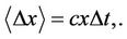 reflecting the (small) bias, or drift, in random steps, (4a)
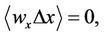 reflecting market participants’ inability to perceive bias in the underlying carries over to an inability to perceive bias in the option price, (4b)
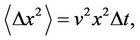 reflecting growth of variance in the random walk.(4c)
Here the parameter c may be positive or negative and reflects the expected drift or trend of underlying stock prices. Note that for this to be a consistent approximation it is required that

meaning that the drift parameter will be small in comparison to volatility, since  (which dovetails with the assumption that it is too small for market makers to take into consideration).
Multiplying (2) by wx, canceling a common factor of N, substituting (3) into (2), replacing the various changes in stock price with their expectations in (4), dividing by  and taking the limit
  leads directly to:
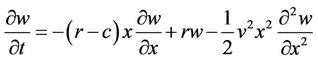 , (5)
, (5)
where c is the implied drift parameter. This is the Extended Black-Scholes (EBS) model. BS’s differential equation can be recovered by setting c to zero. Note that this drift measures the deviation not from current prices, but rather deviation from the interest rate applied to current prices (the arbitrage-free estimate of future prices relative to current prices).
2.2. Solution of the Extended Black-Scholes Equation
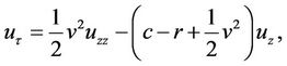
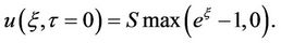
We seek to solve (5) with a boundary condition at maturity (t = t*) given by
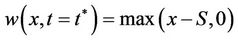 .
.
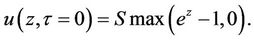
Introducing a change of variables,
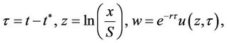
is introduced to remove the non-constant coefficients and exponential growth term, as well as to translate the condition at maturity into an initial condition, giving
with
Changing to a traveling frame of reference 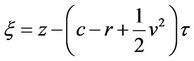 to remove the lowest order z derivative gives a simple diffusion equation:
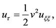
with
The convolution form of the general solution for the diffusion equation is
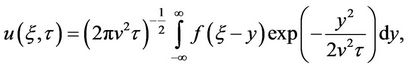
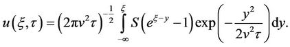
where  is the initial condition. Applying this form of the solution to the initial conditions above, and noting that the integrand will be zero for
  gives
gives
From here, completing the square and using
gives
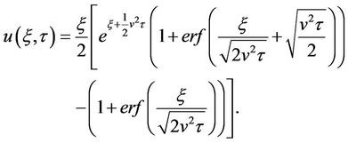
Returning to the original coordinates, simplifying, evaluating at t = 0 and employing the identity
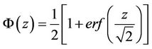 , where Ф is the standard normal cumulative distribution function, gives
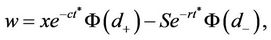 (6)
(6)
where
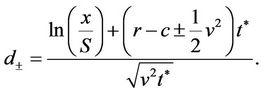
Under the assumption that c = 0 this reduces to the original BS option pricing formula.
3. Data Analysis and Model Competition
In the absence of a market trend (c = 0), with x, r, S and t* assumed known, (6) gives a one-to-one relationship between volatility and option price. Inverting this relationship individually for a series of options, differing only in strike price, often gives a non-constant volatility (the “smile” or “smirk”). However, when c is not zero, how should one proceed? A direct analog to the above procedure would require selecting pairs of options sharing all parameters save strike price, then solving the resulting nonlinear system of equations for v and c. But which pairs should be selected? Or if all possibly pairs are considered, how are results to be interpreted? Are the differences significant? This latter question, in fact, applies also to the volatility smile: given the background variability in underlying stock prices and volatility, are the differences among applied volatilities really significant?
In this paper, an alternate approach is employed following a model competition and selection perspective advanced by Hilborn and Mangel in 1997 [18]. In this approach, model parameters for competing models are fit to all available data using maximum likelihood, cognizant of the fact that there is process variability in the witnessed parameters (e.g. stock prices are clearly not fixed through the course of a day) as well as observational variability (e.g. different market participants may assess volatility using different metrics, over different periods of time, yielding different option prices). Model parameters are chosen to maximize likelihood, and the model which accounts for the most variability among alternative models, with maximum parsimony, should be considered “best”.
3.1. Statistical Methods
The EBS vis-à-vis the BS constitutes a case of nested models, in which the simpler model is realized by a particular choice of parameters in the more complex. A likelihood ratio test may be used to characterize the signifycance of differences between nested models. Assuming both models are fit to data using maximum likelihood, the statistic
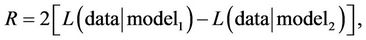
is distributed according to a chi-squared distribution with number of degrees of freedom equal to the difference in numbers of parameters between model 1 (the simpler) and model 2 (the more complex, in which model 1 is nested). Here
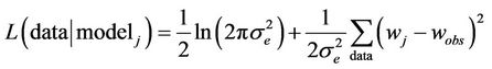
is the negative log-likelihood of model j given the observed data, with wj being the model prediction for the maximum likelihood parameters, wobs being the observed option price and  being the standard deviation of the errors (see [18] for details). Because the difference in these logs is the log of the ratio of the likelihoods, this test is called the likelihood ratio test. The resulting chisquared probability can be viewed as the probability that the more complex model is an improvement over the simpler nested model (that is, the probability that the simpler model’s parameters lie outside the corresponding parametric confidence interval of the more complex model). General wisdom states that parameters should not be added without penalty; the above procedure penalizes the more complex model for its higher number of parameters via the numerical degrees of freedom in the chi-squared distribution.
To determine c and v for each day of data in our EBS model and v for the BS model, we minimize the negative log likelihoods of each over the strike prices for that day. Furthermore, the negative log likelihood of each model is used in the likelihood ratio test, as described above. A corresponding p value was determined from the chisquared distribution with one degree of freedom, indicating the probability that the more complex model (EBS) is a significant improvement over its simpler companion (BS) for that day.
3.2. Data
We use data from the Option Price Reporting Authority (OPRA) for S&P 500 index calls maturing December (19), 2006. The data runs from November 5, 2003 to November 3, 2005. Option Price Reporting Authority provides consolidated option information and is a committee administered jointly by the five option exchanges: AMEX, BOX, CBOE, CBOT, ISE, PCX, PHLX. Our data came indirectly through a third-party vendor. We excluded 5 dates in which the data seemed in error: for the 1325 strike in 2003, November 20, 21, 25, and December 8, 16 and 22; for the 1125 strike, the prices in 2005 of October 24, 25 and 28 and November 2 also seemed probably in error. In the 1150 Strike, the following dates are excluded: 2005 October 19, 24, November 3. We consider only contracts whose strike is between 1125 and 1375, inclusive, and which is a multiple of 25. This has the effect of concentrating on contracts more likely to be liquid and traded, and to eliminate sporadic or illiquid contracts. During this time:
1) The S&P 500 index grew from 1051.81 to 1219.94, with a minimum of 1033.65 (November 20, 2003) and a maximum of 1245.04 (August 3, 2005). The True Range (daily high minus daily low) expressed as a percent of the index value varied from 0.25% to 2.14%, with an average of 0.91% and a standard deviation of 0.37%. (See Figure 2).
2) Average transaction volume per contact grew from about 332 contracts (averaged over 5 working days) to peak of 3476 and ending at 2003 contracts (See Figure 3). This increase is a natural consequence of coming closer to maturity since the shortest dated options are the most traded and liquid.
3) Excluding the 1125 strike contract and certain days due to data issues, implied volatilities varied from 7.57% to 16.05%, with an average of 10.94% and a standard deviation of 1.23%. For each day, the difference between max and min implied volatilities (for days in which more than one contract was traded, and excluding 1125 and 1150 strikes) varied from 0.26% to 6.43%, averaging 1.92% with a standard deviation of 1.04%.
4) We note that the closing price for each option and the index were used. This is a potential source of inconsistency since the last trade for an option contract may not occur at the end of the last moment of stock trading (applicable for the index). Our model, like BS, assumes that the current price of the index is used. Option exchanges generally close before stock exchanges, so closing option and index prices seldom occur simultaneously. Even if the data from within a day were used to synchronize option and index prices, the result may not be as market participants view the market. Market makers may
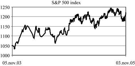
Figure 2. S&P 500 index. The underlying commodity behavior for the options considered, over the time period November 2003 to November 2005.
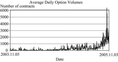
Figure 3. Daily option volume. For each day, the average volume for option contracts in the series studied. As option contracts approach maturity, volume naturally increases since most trading is done in the nearest contract.
well have a backlog of orders in either the option or the shares, such that a market maker could reliably see that the price will move in one direction. Thus the market maker would use an index price in the option formula that differs from the current index price.
3.3. Analysis of Data: Results
To compare the EBS model to the no-drift BS, two fittings are performed. First each day’s closing option prices are fit in the BS to the best implied volatility (one volatility for all options) that maximizes the likelihood of the model given actual option prices. Second, for each day, the EBS is fit for the best combination of drift and implied volatility (one combination for all options on that day) maximizing the likelihood.
To evaluate the results on each day, the worst and average per-day price difference between actual and model are chosen. The error is considered as a percent of the underlying closing index price on that day, with the results summarized in Table 1. The error is approximately halved by the addition of an implied drift parameter. This is true whether looking at the worst price of each day, or the average over all option prices. The ratio of standard deviation to average for the error term does not change significantly when adding a drift parameter.
Using a likelihood ratio test for each day, the drift parameter is seen to have over a 95% chance of improving fit in 297 out of 344 days. Insight can be gained by comparing this statistic with the implied drift for each corresponding day. Figure 4 illustrates that the low chances of improving the model occur on those days in which drift values are close to zero. This is to be expected, given that the probability of improvement depends on where the single parameter BS volatility estimate falls relative to the confidence interval for the drift + volatility estimate for EBS. The EBS fails to be clearly better exactly where its parameters become indistinguishable from the no-drift
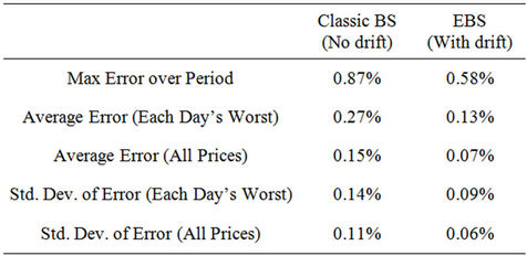
Table 1. Comparison of residuals, Classic BS with and without drift. The modified BS model with drift (called EBS) significantly reduces variability of volatility estimates over the classical BS model. The average variation in each day is generally halved, while the worst fit for each day (an outlier) is also reduced. Further reduction in variability may not be meaningful.
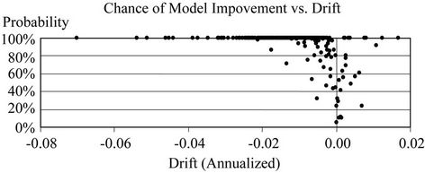
Figure 4. Probability that EBS improves BS. Most often, the chance is 100% that EBS improves BS. The lower probability cases correspond to when the drift is close to zero and the two models are less distinguishable.
BS. This supports the contention that the implied drift parameter significantly improves the model’s fit to actual prices overall.
4. Discussion
The EBS model makes a significant improvement, but perhaps adding more parameters could provide additional significant increases in fit. To the knowledge of the authors, there is no mathematical or statistical method for determining whether or not further parameters could be justified. Rather, practitioners need to look at the data and its context to determine whether or not additional parameters could be warranted. Here it is argued that the closeness of fit using implied volatility-drift in the EBS probably is as close as the data could reasonably allow.
Referring back to Table 1, the average price error for an option in the new model is 0.07%, and the average worst for each day is 0.0013%. Can we expect greater fit than this? These price variations are similar to bid-ask spreads on many illiquid securities. Options have nowhere near the liquidity enjoyed by the underlying index. To attempt any greater fitting of option prices would demand explanations of variations with a magnitude similar to that of bid-ask spreads in the security. This would seem unreasonable for a pricing model that ignores such bid-ask spreads. The conclusion is that the fit offered by the EBS may be as close as is reasonable.
When introducing implied parameters into a model, one should observe how the parameter evolves over time to ensure that the implied parameter is neither too stable nor too erratic. If too stable, the implied parameter probably masks another effect more appropriate for direct modeling. Figure 5 compares the evolution of the implied volatilities that arise from the no-drift (BS) and with-drift (EBS) cases. (Gaps are due to removed data points.) The two volatilities track each other, with the no-drift volatility being higher than the other in practically all cases.
Figures 6 and 7 depict the evolution of the implied drift parameter. Figure 6 displays the parameter itself expressed as a rate similar to interest rates. This is the c
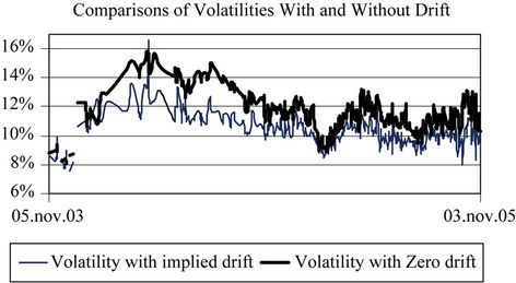
Figure 5. Comparison of implied volatility estimates from EBS and BS. The EBS model’s implied volatility estimate is generally less than that of BS, but the two track each other reasonable well.
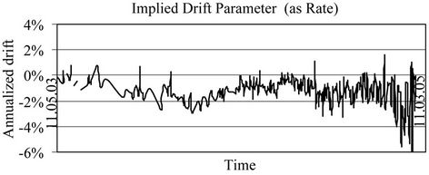
Figure 6. Implied drift in the EBS model (expressed as a rate). The above annualized rates are generally small—the daily price movement would be below what could be detected with statistical studies. The drift parameter becomes erratic closer to maturity as a consequence of annualizing rate on a short-term instrument; this effect is accounted for in the next figure.
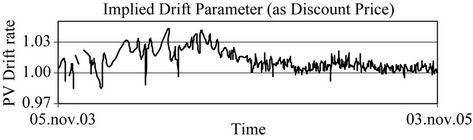
Figure 7. Implied drift in the EBS model (expressed as a discount price). Estimated drift rate data is converted to price data. The implied drift parameter evolves well, neither staying too static nor too fluctuating too erratically.
in Equation (2). As the time to maturity shortens, however, this drift rate becomes erratic, which is typical for any rate that is annualized over progressively shorter time periods; minor discrepancies in price are magnified. To account for this, in Figure 7, the drift parameter is expressed as a price of a zero-coupon bond whose maturity matches that of the option. A zero-coupon bond is a bond with no interest payment. Thus, a zero-coupon bond makes only a single payment, at maturity. The price of such a bond is given by:
where r is the interest rate and t the time to maturity. Given a fixed t, a change in price implies a change in yield. For smaller t, the effect on yield is magnified. When t is very small, say a couple of weeks or less, yield is quite sensitive to price changes, and the effect from day to day can look quite distorted, as in the right end of Figure 6. This price representation displays a variability that dampens as time approaches maturity. This confirms the contention that the drift reflects price movements (either perceived by market participants or latent in the market) since over shorter horizons, lower price drifts appear.
While yield is typically express as a percent return per year, the implied drift parameter in Figure 7 can be expressed per day, by taking the difference of the price from 1.00 and dividing it by the number of days to maturity. This is the average daily drift implied by market prices. Over our sample, this varied from −0.0042% to 0.0204%, with an average of 0.0033% and standard deviation of 0.0028%. These are exceptionally small numbers which could never be confirmed from historical analysis. This conclusion is consistent with a result from Brownian motion: that over short periods any drift effects are completely dominated by the noise or random effects (See [19] p. 656 for further discussion). Using drift as an implied parameter implicitly allows it to vary moment to moment (or, in our case, day to day), and thus it would be difficult if not impossible to detect. Perhaps if any particular drift were valid over a longer period of time (say until maturity), then there might be a chance to confirm it with a historical study, but this is not the case. Given the momentary nature of an implied parameter, there is no real hope of confirming the validity of any particular drift measurement. Nonetheless, the effect over time until maturity is significant and affects option pricing.
5. Conclusions
In this paper, the Black-Scholes option pricing model is modified to have a free drift parameter alongside volatility. Similar to the original BS work, the ensuing differential equations are developed, and a closed-form solution for this model is derived, with the resulting model referred to as the Extended Black-Scholes (EBS). Rather than fitting the new drift parameter historically, it is treated as an implied parameter, like volatility. Using historical data, each day’s closing volatility smile is best-fit to an implied volatility-drift combination. A likelihood ratio test indicates that the implied drift parameter significantly improves the fit of the EBS model as compared with the BS model. It is argued that any better fit may not be justified, since the remaining unexplained differences between EBS and option prices are very similar to bid-asked spreads for securities whose liquidity is comparable to that of options. Furthermore, the small size of the daily drift parameter indicates that it would be unlikely to be uncovered during historical analysis.
The new drift parameter may be interpreted in one of two ways: it may be an actual trend that is too small for market participants to observe; or it may be a small trend perceived by market participants and driving their prices, whether or not this drift actually exists in the market. These interpretations represent two opposing views of pricing theory: either security prices arise strictly from underlying market dynamics, or arise from perceptions of market players. It is interesting that historical testing cannot be used to resolve this debate, since the EBS is an option pricing model that can explain prices as much as justifiable, while accommodating either assumed cause.
REFERENCES
- B. Dupire, “Pricing with a Smile,” Risk, Vol. 7, No. 1, 1994, pp. 18-20.
- F. Black and M. S. Scholes, “The Pricing of Options and Corporate Liabilities,” Journal of Political Economy, Vol. 81, No. 3, 1973, pp. 637-654. doi:10.1086/260062
- R. Merton, “Option Pricing When Underlying Stock Returns Are Discontinuous,” Journal of Financial Economics, Vol. 3, No. 1-2, 1976, pp. 125-144. doi:10.1016/0304-405X(76)90022-2
- F. Black, “The Pricing of Commodity Contracts,” Journal of Financial Economics, Vol. 3, 1976, pp. 167-179. doi:10.1016/0304-405X(76)90024-6
- J.-P. Bouchaud and M. Potters, “Back to Basics: Historical Option Pricing Revisited,” Philosophical Transactions of the Royal Society, Vol. 357, No. 1735, 1999, pp. 2019-2028.
- E. Derman, “Regimes of Volatility,” Risk, Vol. 4, 1999, pp. 55-59.
- E. Derman and I. Kani, “Riding on a Smile,” Risk, Vol. 7, No. 2, 1994, pp. 32-39.
- M. Rubinstein, “Implied Binomial Trees,” Journal of Finance, Vol. 49, No. 3, 1994, pp. 771-818.
- L. Andersen and R. Brotherton-Ratcliffe, “The Equity Option Volatility Smile: An Implicit Finite-Difference Approach,” Journal of Computational Finance, Vol. 1, No. 2, 1997, pp. 5-38.
- J. C. Hull and A. White, “An Analysis of the Bias in Option Pricing Caused by a Stochastic Volatility,” Advances in Futures and Options Research, Vol. 3, 1988, pp. 29- 61.
- S. L. Heston, “A Closed-Form Solution for Options with Stochastic Volatility with Applications to Bond and Currency Options,” Review of Financial Studies, Vol. 6, No. 2, 1993, pp. 327-343. doi:10.1093/rfs/6.2.327
- D. S. Bates, “Jumps and Stochastic Volatility: Exchange Rate Processes Implicit in Deutsche Mark Options,” Review of Financial Studies, Vol. 9, No. 1, 1996, pp. 69- 107. doi:10.1093/rfs/9.1.69
- B. Dupire, “A Unified Theory of Volatility,” Working Paper, 1996.
- A. Lipton and W. McGhee, “Universal Barriers,” Risk, Vol. 15, No. 5, 2002, pp. 81-85.
- M. Britten-Jones and A. Neuberger, “Option Prices, Implied Prices Processes, and Stochastic Volatility,” Journal of Finance, Vol. 55, No. 2, 2000, pp. 839-866. doi:10.1111/0022-1082.00228
- G. Blacher, “A New Approach for Designing and Calibrating Stochastic Volatility Models for Optimal DeltaVega Hedging of Exotic Options,” Conference Presentation at Global Derivatives and Risk Management, Juanles-Pins, 26 June 2002.
- D. Brigo and F. Mercurio, “A Mixed-Up Smile,” Risk, Vol. 13, No. 9, 2000, pp. 123-126.
- R. Hillborn and M. Mangel, “The Ecological Detective: Confronting Models with Data,” Princeton University Press, Princeton, 1997.
- R. L. McDonald, “Derivative Markets,” 2nd Edition, Addison Wesley, New York, 2006.
NOTES
*Corresponding author.