Theoretical Economics Letters
Vol. 2 No. 5 (2012) , Article ID: 25818 , 6 pages DOI:10.4236/tel.2012.25094
Is Product of Two Convex Functions Necessarily Convex? A Case of the MRP Curve
1Department of Economics, Clarion University of Pennsylvania, Clarion, USA
2Department of International Business, Ming Chuan University, Taipei, Taiwan
3Sanchez School of Business, Texas A & M International University, Laredo, USA
4Department of Marketing, Clarion University of Pennsylvania, Clarion, USA
Email: hungkuen@gmail.com
Received July 25, 2012; revised August 26, 2012; accepted September 27, 2012
Keywords: Theoretical MRP; Empirical MRP; Concavity; Convexity; Linearity
ABSTRACT
The curvature of the marginal revenue product curve plays an important role in most theoretic microeconomic models since it determines the size of profit contribution to an employer and optimality conditions of solutions. There are many well established introductory and intermediate microeconomic textbooks portray marginal revenue product curves as linear or concave to the origin. In nearly all cases, the MRP cannot be linear, nor can it be concave. In this analysis, most of the well-known production functions generate convex MRP curves.
1. Introduction
Input hiring decisions play an important role in microeconomic theory. These decisions are based on the monetary contribution of a variable input to the firm compared with its cost. In a competitive output market, it is known as the value of the marginal product (VMP), whereas in a monopoly market, the additional monetary contribution is often referred to as the marginal revenue product (MRP). These two concepts, VMP and MRP, are equal in the competitive output market as its output price equals marginal revenue. This paper shows first that the MRP curve cannot be linear in input factor although it is often drawn as such in many microeconomics textbooks. As is shown by Yang, Means, and Moody [1], for a given domain, the concavity or convexity property may not be preserved beyond functional addition. The MRP curve cannot be concave to the origin, due to the fact that even the product of two concave functions may not necessarily be concave.
In this paper, we analyze the shape of the MRP curve mathematically, then present a set of simulations for a variety of well-known production functions frequently used in microeconomics textbooks. The non-concavity of the MRP curve (especially in production stage II) is witnessed in these simulations. The curvature of the MRP curve plays an important role in most standard microeconomic models (see e.g. Takayama [2], Baumol and Klevorick [3]) in determining the characteristics of optimal solutions.
2. Shapes of MRP Curves
Given that the marginal revenue curve of a linear demand is twice as steep, the curvatures of the MRP and VMP are qualitatively similar. Thus, our paper focuses on the shape of MRP curves. The quintessence of the MRP curve is the product of two functions: Marginal product of labor  and marginal revenue
  in the output market. To investigate the shape of the MRP curve, we start with
 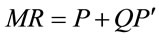 or
or 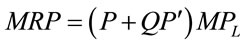 where
where  and
and :
:
 (1)
(1)
where  and
and  indicates decreasing marginal product of labor and
 .
.
The curvature of the MRP curve can be determined by the second derivative with respect to labor or
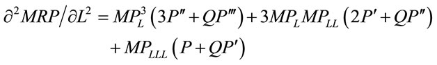 (2)
(2)
where  and
and  is the second derivative of
 .
.
Note that the sign is not easily amenable to the analysis: It requires . Tables 1 and 2 illustrate the shapes of the MRP curve in the cases of linear demand and constant elasticity demand. Given a linear demand function and a standard concave production function Q, with some fixed capital, K, the shape of
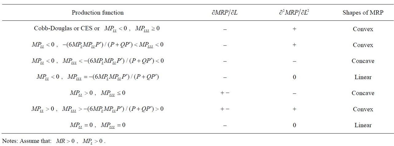
Table 1. Shapes of MRP curves: Linear demand ,
,  ,
, .
.
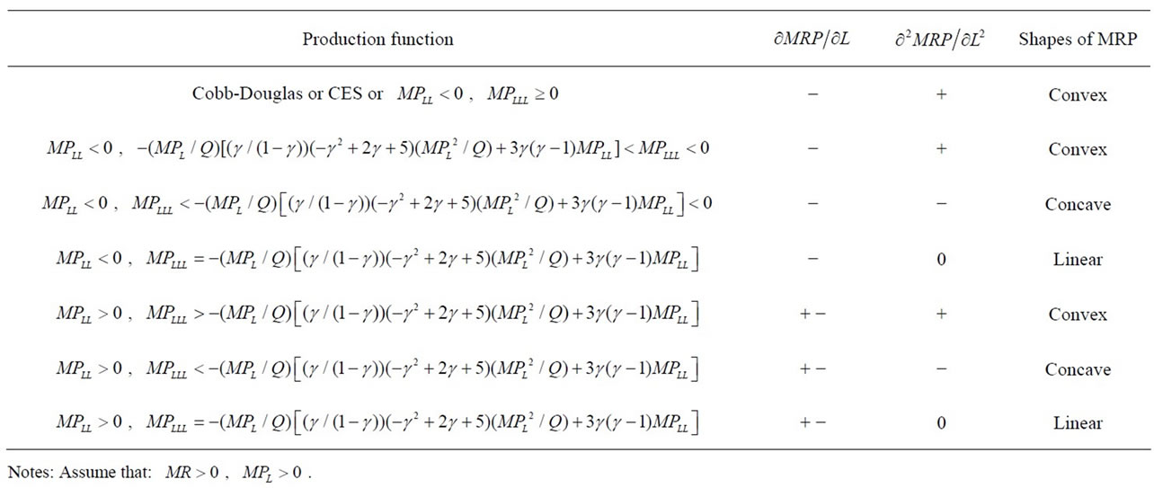
Table 2. Shapes of MRP curves: Constant elasticity demand ,
,  ,
,  ,
,  ,
, .
.
MRP curve is determined by (1) the  function which is convex with respect to L, and (2) the
  function. Since many well-known production functions, such as the Cobb-Douglas [4], CES (see Arrow, Chenery, Minhas and Solow [5]), VES (see Mukerji [6] and Revankar [7]) and Translogarithm (see Christensen, Jorgenson and Lau [8]), have rather convex
 , it is not likely that the product of two convex functions is linear or concave curves.
For a constant elasticity demand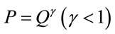 , it can be shown readily that
 ,
,  , and
, and . Without the knowledge on the production function, signs of
  and
and  alone are not sufficient to determine the shape of MRP curve.
The MRP curves, for almost all possible cases, can be neither linear nor concave to the origin in terms of the variable input. They cannot be linear because the product of even two linear functions (one is the function of the other) cannot be linear.
In order to explore the possible shapes of MRP curves, the following production functions are examined:
Cobb-Douglas
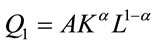 (3)
(3)
Cubic
 (4)
(4)
Quadratic
 (5)
(5)
Constant Elasticity of Substitution (CES)
 (6)
(6)
Variable Elasticity of Substitution (VES)
 (7)
(7)
Variable Elasticity of Substitution (VES)
 (8)
(8)
Translogarithmic Production Function
 (9)
(9)
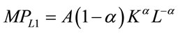
2.1. Case I: MRP Curves in a Perfectly Competitive Output Market
In perfect competition, the VMP or MRP is simply the product of a constant price or  and
and . As a consequence, the MRP has the exact curvature of the
 . Only when
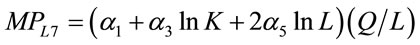
 is linear in L, can one draw a corresponding linear MRP curve. The
  for a given K corresponding to the previously specified production functions have the following forms1
 (10)
(10)
 (11)
(11)
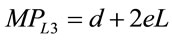 (12)
(12)
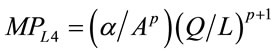 (13)
(13)
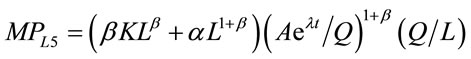 ) (14)
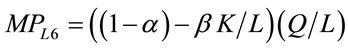 (15)
(15)
 (16)
(16)
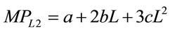
Hence, a linear MRP (VMP) curve is logically inconsistent except in the case of a quadratic production function (Q3) whose  is a linear decreasing function in L. In such a case, a liner MP times a constant price gives rise to a linear VMP (MRP) curve. Notice that except in the case of the cubic production function with a negative coefficient on the cubic terms in which APL and
  are concave to the origin, all other MRP (VMP) curves are convex.
In general, the MRP decreases as the input increases. Strictly speaking, a linear MRP curve from a quadratic production function cannot reflect characteristics of the well-behaved production functions. Using the parameters of well-known production functions2 (Cobb-Douglas, Constant and Variable Elasticity of Substitution (CES, VES) and Translogarithm) and assuming the simplest case of linear demand function3, Figures 1-7 illustrate specific VMP (MRP) curves. These curves cannot be concave to the origin for most empirically relevant parameters.
2.2. Case II: MRP Curves in Imperfectly Competitive Output Markets
The MRP of labor in imperfectly competitive markets is the product of  and
and . As is true with the VMP curves, most MRP curves cannot be linear. The fundamental difference from the previous case is that MR curve is no longer a constant. It is a linear function of output, which is concave to L. The MRP curves are shown in Figures 8-14. Again, the only exception found
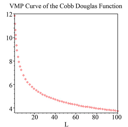
Figure 1. 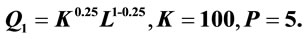 Notes: Estimated parameters are taken from Douglas [9].
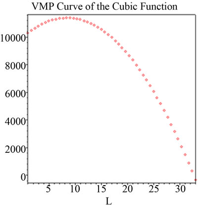
Figure 2.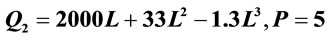 .
.
is the case of a constant  (linear production function) with a linear demand function. It is to be pointed out that product of a linear
  function (convex with respect to L) and a convex
  (in most well-known cases) is not likely to be concave. A concave MRP reflects logical inconsistency in nearly all cases5.
Examination of undergraduate textbooks that cover microeconomics indicates a range of approaches in discussions of the MRP curves. Of the 61 texts surveyed, most texts present the logically erroneous and empirical infeasible concave MRP curve. Only 15 of 61 texts (24.59%) illustrate the MRP curves correctly, as convex to the origin6. In particular, of the prominent texts including those authored by Nobel laureates in Economics, Price Theory by Milton Friedman [12] and Economics by Paul A. Samuelson and William D. Nordhaus [13] draw MRP curves correctly.
Figure 3. .
.
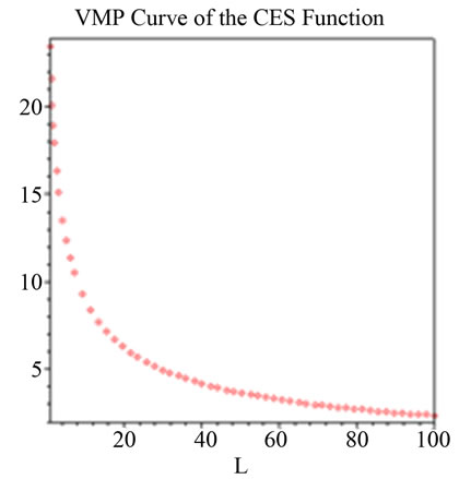
Figure 4. Q4 = 1.016 (0.464−0.236 + (1 – 0.464)K−0.236)−1/0.236, K = 100, P = 5; Notes: Estimated parameters are taken from Arrow, Chenery, Minhas and Solow [5].
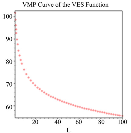
Figure 5. Q5 = 6.2705e0.0183t ((1 + 6.7501) KL6.7501 – 0.3025L(1 + 6.7501))1/(1 + 6.7501), K = 100, t = 25, P = 5. Notes: Estimated parameters are taken from Lovell [10].
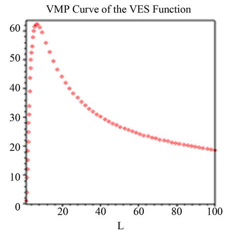
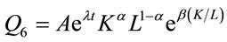
Figure 6. Q6 = 21.5091e0.0181tK0.4657L(1 - 0.4657)e−2.5361(K/L), K = 3, t = 25, P = 5. Notes: Estimated parameters are taken from Lovell [10].
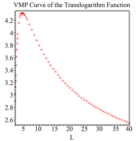
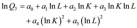
Figure 7. lnQ7 = −0.156lnL + 0.721lnK – 0.057lnKlnL + 0.063 (lnK)2 + 0.062 (lnL)2, K = 30, P = 5; Notes: Estimated parameters are taken from Humphrey and Moroney [11].
3. Conclusions
We have simulated VMP and MRP curves with empirically relevant parameters of demand and production,
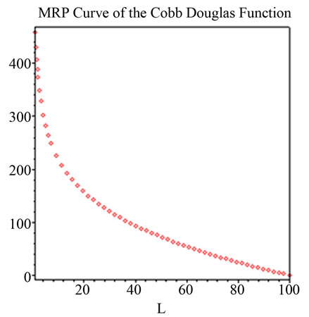
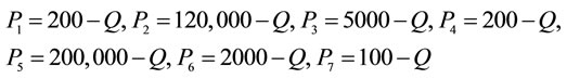
Figure 8. Q1 = K0.25 L1 − 0.25, K = 100, h = 200, i = 1 (P = 200 − Q); Notes: Estimated parameters are taken from Douglas [9].
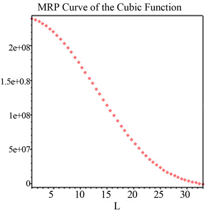
Figure 9. Q2 = 2000L = 33L2 – 1.3L3, h = 120,000, i = 1 (P = 120,000 − Q).
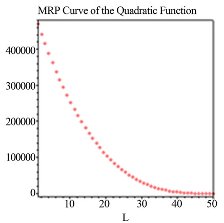
Figure 10. .
.
which indicate that most of MRP curves are convex to the origin. This finding is quite in contrary to the straight or concave MRP curves often found in textbooks.
The fact of errors in some 75.41% of textbooks is important for at least two reasons. The first is simple accuracy and consistency. A concave VMP (MRP) curve is possible only with the cubic function in perfect competetion. As for MRP curves, a linear or concave one is a mathematical oddity or impossibility. Even the MRP curve of the cubic production function is convex in the efficient production range where the marginal product is relatively small. The second has to do with the rhetoric of economics. As McCloskey [14] discusses at length, there are many rhetorical devices used in economics just to simplify a concept. Potentially damaging rhetoric exists where we try too hard to “twist” the curves to illustrate optimum labor hiring.
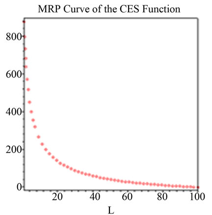
Figure 11. Q4 = 1.016 (0.464−0.236 + (1 – 0.464)K−0.236)−1/0.236, K = 100, h = 200, i = 1 (P = 200 − Q); Notes: Estimated parameters are taken from Arrow, Chenery, Minhas and Solow [5].
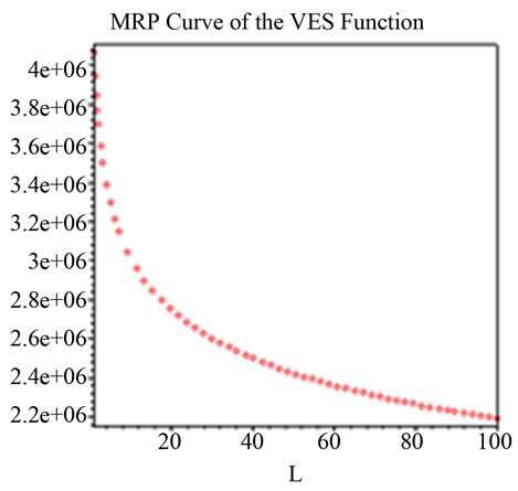
Figure 12. Q5 = 6.2705e0.0183t((1 + 6.7501)KL6.7501 − 0.3025L(1 + 6.7501))1/(1 + 6.7501), K = 100, t = 25, h = 200000, i = 1 (P = 200,000 − Q); Notes: Estimated parameters are taken from Lovell [10].
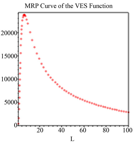
Figure 13. Q6 = 21.509e0.0181tK0.4657L(1 − 0.4657)e−2.5361(K/L), K = 3, t = 25, h = 2000, i = 1 (P = 2000 − Q); Notes: Estimated parameters are taken from Lovell [10].
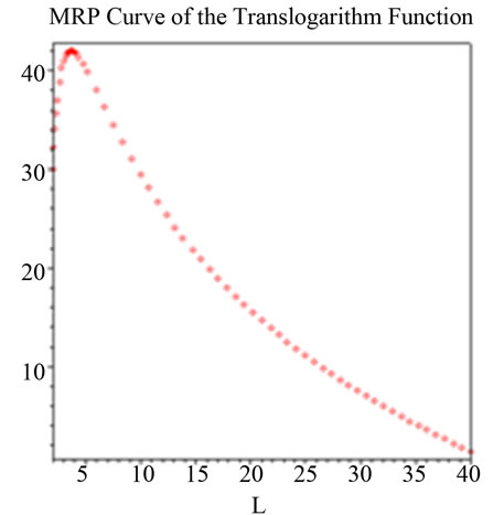
Figure 14. lnQ7 = −0.156lnL + 0.721lnK − 0.057lnKlnL + 0.063(lnK)2 + 0.062(lnL)2, K = 30, h =100. i =1 (P = 100 − Q); Notes: Estimated parameters are taken from Humphrey and Moroney [11].
As the article makes clear, under reasonable parametric limits, the MRP curve should be convex to the origin. Finally, from the viewpoint of policy implications, a convex MRP may well translate into hiring fewer workers if wage rate is relatively high: a disturbing phenomenon facing developed economies nowadays.
REFERENCES
- C. W. Yang, D. B. Means and G. E. Moody, “Tax Rates and Total Tax Revenues from Local Property Taxes,” Public Finance Quarterly, Vol. 21, No. 4, 1993, pp. 355- 377. doi:10.1177/109114219302100401
- A. Takayama, “Behavior of the Firm under Regulatory Constraint,” The American Economic Review, Vol. 59, No. 3, 1969, pp. 255-260.
- W. J. Baumol and A. K. Klevorick, “Input Choices and Rate-Of-Return Regulation: An Overview of the Discussion,” The Bell Journal of Economics and Management Science, Vol. 1, No. 2, 1970, pp. 162-190. doi:10.2307/3003179
- C. W. Cobb and P. H. Douglas, “A Theory of Production,” American Economic Review, Vol. 18, No. 1, 1928, pp. 139-165.
- K. J. Arrow, H. B. Chenery, B. S. Minhas and R. M. Solow, “Capital-labor Substitution and Economic Efficiency,” The Review of Economics and Statistics, Vol. 43, No. 3, 1961, pp. 225-250. doi:10.2307/1927286
- V. Mukerji, “A Generalized S.M.A.C. Function with Constant Ratios of Elasticity of Substitution,” Review of Economic Studies, Vol. 30, No. 3, 1963, pp. 233-236. doi:10.2307/2296324
- N. S. Revankar, “A Class of Variable Elasticity of Substitution Production Functions,” Econometrica, Vol. 39, No. 1, 1971, pp. 61-71. doi:10.2307/1909140
- L. R. Christensen, D. W. Jorgenson and L. J. Lau, “Transcendental Logarithmic Production Frontiers,” Review of Economics and Statistics, Vol. 55, No. 1, 1973, pp. 8-45. doi:10.2307/1927992
- P. H. Douglas, “Are There Laws of Production?” American Economic Review, Vol. 38, No. 1, 1948, pp. 1-42.
- C. A. K. Lovell, “Estimation and Prediction with CES and VES Production Functions,” International Economic Review, Vol. 14, No. 3, 1973, pp. 676-692. doi:10.2307/2525980
- D. B. Humphrey and J. R. Moroney, “Substitution among Capital, Labor, and Natural Resource Products in American Manufacturing,” Journal of Political Economy, Vol. 83, No. 1, 1975, pp. 57-82. doi:10.1086/260306
- M. Friedman, “Price Theory,” 2nd Edition, Aldine Publishing Company, New York, 1976.
- P. A. Samuelson and W. D. Nordhaus, “Economics,” 17th Edition, McGraw-Hill, New York, 2005.
- D. N. McCloskey, “The Rhetoric of Economics,” 2nd Edition, University of WI Press, Madison, 1998.
NOTES
1Differentiate Equations (3)-(9) with respect to L, we could obtain Equations (10)-(16).
2Simulation of Figure 8 is based on well-known estimation by Douglas [9]. The parameters on quadratic and cubic production functions are quite common, i.e., e ≤ 0 and c ≤ 0 as in many textbooks. The CES production functions are from Arrow, Chenery, Minhas and Solow [5]; VES production functions are from Lovell [10] and the translogarithmic production functions are from Humphrey and Moroney [11].
3The demand functions used with the corresponding production func- tions to calculate the MRP are the following:
4The  for a given K corresponding to the previously specified production functions (Equations (3)-(9)) are Equations (10)-(16)).
5Note that even a cubic production function with negative coefficient on cubic term must generate convex MRP curve in the efficient production stage where marginal product approaches zero (Figure 9).
6Names and authors of the textbooks, being lengthy, are available upon request.