ABSTRACT

The paper provides a model that explains mixed land use patterns in urban areas. The paper contains a proof of the existence of competitive market equilibrium in a market for land in a small zone where more than one land use may be present. The model includes the possibility that external effects (both negative and positive) exist among the land uses. Brouwer’s fixed point theorem is used for the proof. Conditions are derived in which mixed land use is an equilibrium pattern in a monocentric city.

1. Introduction

Fifty years ago William Alonso published the short version of his classic theory of location and land use [1]. That article presented the theory of bid rent curves, and concluded that the land use pattern of the monocentric city would consist of a set of von Thűnen concentric rings [1, p. 155].

We now have, conceptually, families of bid rent curves for all three types of land uses. We also know that the steeper curves will occupy the more central locations. Therefore, if the curves of the various users are ranked by steepness, they will also be ranked in terms of their accessibility from the center of the city in the final solution. Thus, if the curves of the business firm are steeper than those of residences and the residential curves steeper than the agricultural, there will be businesses at the center of the city, surrounded by residences, and these will be surrounded by agriculture.

Alonso’s theory remains at the core of models used to understand spatial patterns in urban areas. Fujita [2] provides a complete presentation of models in the Alonso tradition. The purpose of this paper is to present an extension of the Alonso model to provide an explanation for the fact that urban land uses are mixed and the landuse pattern does not conform to neat von Thűnen rings.

This paper begins by considering market-determined land use allocation in a small zone in an urban area. The zone is not subject to zoning or other forms of control on land use allocation, and includes the possibility that land values in a particular use depend upon the amounts of land in the zone devoted to other uses. In other words, the model includes external effects of a particular form.

The final section in this paper adds location (distance to the central business district) to the model, which generates the possibility (for example) that land use is exclusive, then mixed, and then exclusive as distance to the CBD increases. This result provides an explanation for mixed land use that is complementary to the model developed by Wheaton [3].

The paper makes use of Brouwer’s fixed point theorem, which is stated in a variety of equivalent forms. Varian [4, p. 320] states the theorem as follows:

If f: is a continuous function from the unit simplex to itself, there is some x in such that x = f(x).

Here S is a set of real numbers with dimensions with a range over the unit simplex.

Debreu [5, p. 26] states the theorem as: “If S is a non-empty, compact, convex subset of Rⁿ, and if f is a continuous function from S to S, then f has a fixed point.” Alternatively, Mendelson [6] provides a clearer statement of the theorem. Define the unit cube in n dimensional space, denoted Iⁿ, as the set of points whose coordinates satisfy the inequalities, for. Mendelson [6, p. 125] states: “Let f: Iⁿ → Iⁿ be continuous. Then there is a point z in Iⁿ such that”. Clearly the unit cube includes the case of for x_i that satisfies the above inequality.

Consider an introductory example in which there are two types of land uses, residential and commercial. The bid-rent function for residential use is simply a function of distance to the central business district (CBD);

with u as distance to the CBD. However, suppose that bid-rent for commercial use is a function both of distance to the CBD and the proportion of land in a small zone that is dedicated to residential use. Commercial users of land value access to customers, so

where q is the proportion of land in the zone devoted to residential use. Assume that the bid-rent function for commercial use has a greater intercept and a steeper slope than does the residential bid-rent function, and that γ is greater than zero. The CBD is defined as the area where bid-rent for commercial land exceeds bid-rent for residential land (even if q = 0). This distance is denoted u^*. Beyond distance u^*, exceeds, so some land is devoted to residential use. How much land will be devoted to residential use? The answer is: enough q (proportion of land in residential use) to make

Residential land in the zone boosts the value of the land devoted to commercial use just enough to establish equality between the two bid-rent levels. And this is a stable equilibrium because there is no further incentive to convert the use of land.

As distance to the CBD increases commercial bid-rent (holding q constant) continues to decline more rapidly than residential bid-rent, so the proportion of land devoted to residential use increases with distance and land use continues to be mixed. Eventually a distance u^** may be reached at which the bid-rent for residential use equals the bid-rent for commercial use even if the proportion of land in residential use is 1.0; i.e.,

Beyond this distance land is devoted exclusively to residential use. The resulting market equilibrium land rent profile is shown in Figure 1.

2. Microeconomic Foundations

This paper is concerned with the market for land in a zone of finite size located in an urban area. The zone is occupied by households and/or firms, and the total amount of land occupied by these actors equals the total amount of land in the zone (L). In this section it is assumed that transportation costs are identical from all locations in the zone. Consider the zone in partial equilibrium.

Household utility is a function of a composite good (x), land (l), and possibly the percentages of land in the zone occupied by residential and other types of users of land (vector q). Households who choose to locate in the zone do so because the level of utility achieved is equal to the level (Ū) that can achieved elsewhere, so for household i,

(1)

The marginal effects of x and l on U are positive, and the marginal effects of externalities q can be of either sign. Households maximize utility subject to a budget constraint, where w is income, R is the land rent in the zone, and tu is commuting cost (at distance u at cost per mile t). The indirect utility function can be derived and stated as

(2)

Bid-rent for the household is

(3)

Bid-rent is completely determined if the arguments in this function are given values.

The expenditure function for household i is

(4)

so the (compensated) demand for land is

If p_x, and w are fixed, q in the zone is given, and Ū_i is the required level of utility in the zone, then bid rent and the amount of land demanded by household i are determined.

Bid rent as a function of distance is found by totally differentiating the indirect utility function and solving for

(where for an increase in distance)with the result that, for,

(5)

Bid rent declines with distance because t and are positive and is negative. The relationship between bid rent and the percentage of land occupied by other types of users of land also can be found by totally differentiating the indirect utility function, with the result that, for,

(6)

The sign of is negative, and can be positive, zero, or negative.

If all households in the urban area (and the zone) are identical, then the number of households in the zone (n) is

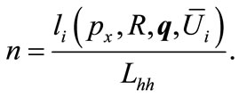(7)

The total amount of land in the zone occupied by households is

(8)

Now consider firms that may occupy sites in the zone. A simple characterization of firms is used here. Firms produce output with constant returns to scale and fixed factor proportions and earn zero economic profit. Firms employ Ē workers and occupy ĺ_f units of land. The amount of output that these inputs produce may vary depending upon the land use pattern in the zone in which the firm is located. The profit function for a firm is

(9)

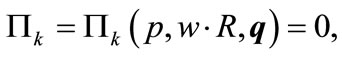
where p is the price of output and w is the wage paid to workers. Output and profit are functions of land uses in the zone for reasons that are discussed in the next section. The relationship between bid rent and land uses can be found by totally differentiating the profit function. Setting, the results are

(10)

and

(11)

The marginal effect of land rent on profits is negative, and the marginal effects of land uses on profits can be of either sign.

3. The Model

The model considers a zone in an urban area that potentially can be used for one or more uses such as residential, commercial, industrial, and so on. It is assumed that the zone is small; the shadow value of land in the zone does not change as the size of the zone is increased marginally. The zone is small enough that its location vis-à-vis the rest of the urban area is considered to be identical for all points in the zone. The zone is of a size that external effects caused by mixed land uses in the zone can matter. The microeconomic models of consumer and firm in the previous section include the possibility that land use in the zone affects bid rent. The zone is not subject to zoning or other controls on land use. The zone may be several blocks, or it may be somewhat larger. Some empirical applications of the model are based on block data.

The proportion of the zone that is in use i is q_i, and the land value per unit of land in use i is, where q is the vector of the proportion of land uses in the zone, and is a real-valued continuous function (that need not be differentiable). The elements of q are proportions of land used by households and firms, as discussed in the previous section. The set of values for q sums to 1.0 and is convex. The land value functions can assume many specific forms. The signs of marginal effects are ambiguous. Consider commercial activities such as retail store, for example. The first store in the zone on a predominantly residential block enjoys advantages for which the owner is willing to pay a premium. Additional stores in the zone increase the competition and lower the store owner’s bid for the land. Alternatively, there may be economies of agglomeration in store location—the shopping center effect. In this case the store owners may bid more for land in zones with other stores. The store owner’s bid for land may also be affected by other land uses. Greater land devoted to residential use may increase the store owner’s bid for land (access to customers), and they may bid less for land in zones with greater amounts of industrial use. It is also possible that the store owner’s bid is unaffected by the land-use composition of the zone, in which case the marginal effects are zero and land value in commercial use is determined entirely by the location of the zone vis-à-vis the rest of the urban area. Owners of land used for residential purposes may bid more for land if the proportion in residential use increases, or they may value immediate access to commercial activities and employment. Owners of land for industrial purposes may value proximity to supporting commercial activities and workers, or there may be agglomeration economies in industrial land use that govern the bids for land.

The primary question that is solved in this paper is whether a market equilibrium set of land-use proportions (the q’s) exists. The basic approach to the existence proof can be seen in the case of two possible land uses. Indeed, the case of two land uses is quite pertinent for many applications of the model.

4. The Case of Two Land Uses

Consider the case of two land uses, such as residential use and commercial use. There are two land-use proportions, q₁ and q₂, which sum to 1.0. Because there are only two land uses, the model needs to determine only q₁, which shall be denoted q. There are two land value functions;

The variable q varies from 0 to 1.0, so it is an ideal variable for an application of Brouwer’s fixed point theorem. The theorem requires a function of q that maps q into another continuous variable that varies from 0 to 1.0.

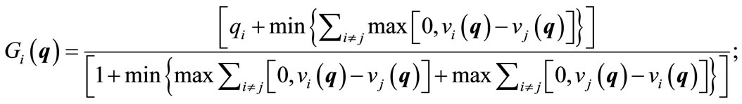
Consider the following function that meets this requirement;

(12)

i = 1, 2 and j = 1, 2.

G(q) is a real-valued continuous function that maps the unit line to itself. G(q) is a fictitious quantity adjustment equation that is analogous to the fictitious price adjustment equation that is used in proofs of the existence of an equilibrium vector of relative prices in a competitive market economy, as in Arrow and Debreu (7). Brouwer’s fixed point theorem states that there exists q = q^* such that

(13)

Equation (13) implies that

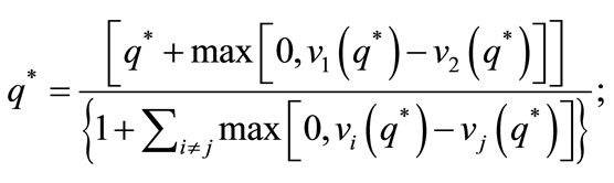(14)

i = 1, 2 and j = 1, 2.

There are three cases to examine in which Equation (14) is satisfied.

If, then:

If, then, and:

If, then.

The first condition states that, if the land use number one does not exist in the zone, the value of the land in the alternative use must be equal to or greater than value in use one. This makes the numerator of the right-hand side of Equation (14) equal to zero.

The second condition states that, if both uses exist in the zone, then the land values for the two uses must be equal. This makes the right-hand side of Equation (14) equal to q^* between 0 and 1.0. The proof is by contradiction. If the two land values are not equal, either

If the value of land in the first use exceeds value in the alternative use by a positive amount x, then we have

which cannot hold for. If the value of land in the second use exceeds the value in the first use by positive amount y, then

which cannot hold for

The third condition states that, if land use number one is the only land use in the zone, then the value of land in that use is equal to or greater than the value of the land in the alternative use, which makes the right-hand side of Equation (14) equal to 1.0.

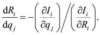
The existence of at least one market equilibrium q has been established. However, not all equilibria are stable. Stability requires that for the case in which mixed land use exists. (The delta notation is used for a small finite change in q and resulting finite change in land value because the land-value functions are continuous but not necessarily differentiable.) If this stability condition does not hold, then the market activity will increase (decrease) q up to the point at which the stability condition is satisfied or q = 1 (q = 0). This stability condition also applies if q = 1 or q = 0 and it so happens that. The other side of the stability condition is, which is an identical condition. The more general statement of the condition is, i ≠ j.

Solution of the model can be illustrated through a simple example. Suppose that v₁ = a + bq and v₂ = c + eq. The external effects, b and e, can of either sign. In this case stable equilibria exist in the following cases:

if,

if, and

if and.

If, then if and if.

Either or can be an equilibrium if and.

5. The Case of Three or More Land Uses

The case of three land uses adds complexity to the analysis. Now there are three land uses such that; i = 1, 2, 3. And there are three land value functions; i = 1, 2, 3. The problem is to determine the equilibrium values for two of the land uses.

Two fictitious quantity adjustment equations are specified as follows. These equations are analogous to Equation (12) above.

j = 2, 3,(15)

and 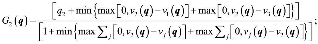j = 1, 3.(16)

Equations (15) and (16) are functions from the unit simplex q to itself, and are continuous. Brouwer’s fixed point theorem states that there exists a vector q such that

(17)

As in the case of two land uses, there are three cases to consider for each equation of equilibrium.

If then and, and similarly for q₂. These conditions are needed to make the numerators of Equations (15) and (16) equal to zero.

If, then

andor and

or and (18)

Similar conditions hold for q₂. These conditions mean that the numerator of the right-hand side of Equation (15) equals q₁ and that the denominator equals 1.0.

Lastly, if q₁ = 1, then the land value in use number one is equal to or exceeds land value in either of the alternative use. Satisfaction of this condition means that the numerator and denominator of Equation (15) are both equal to 1.0. A similar condition holds for land use number two.

A stability condition applies to each of the land uses that is similar to the condition in the case of two land uses. An equilibrium in which the land use in question is between zero and 1.0 requires that there is no incentive to convert some of that land to another use. The general statement of the stability condition applies;,

. As noted in the case of two land uses, the stability condition is also needed if it so happens that land values for two land uses are equal and one of those land uses does not exist in the zone.

Now consider the general case of N land uses. This case adds little that has not already been discovered in the case of three land uses. There are now N land uses that sum to 1.0, and there are N land value functions of the form. And now fictitious quantity adjustment equations are specified of the form:

i, j = 1, ···, N.(19)

The analogous three cases hold for each of the land uses; land use can be zero, between zero and 1.0, or 1.0.

6. Addition of Location to the Model

A useful extension of the model is to assume a monocentric city in which bid rents decline with distance to the central business district (CBD). A standard result in urban economics, first stated by Alonso [1] and demonstrated rigorously by Fujita [2, p. 129] is that:

Assuming that the set of bid rent functions can be ordered according to their steepness, we obtain neat results: Both the equilibrium land use and optimal land use exist uniquely, and they can be depicted by a set of Thünen rings surrounding the CBD.

This configuration is at variance with the facts; land use in real cities is mixed. As in the standard modelworkers who work in the CBD are paid a wage, but must also pay commuting costs. Residential bid rents decline with distance to the CBD as a result. In general, firms occupy the area near the CBD, land is mixed at intermediate distances, and land is exclusively in residential use at greater distances. The model in this section is based on these ideas; residential bid rents decline with distance to the CBD because of commuting costs, and the productivity of a firm declines with distance to the CBD because of declining agglomeration effects. Workers who work near home earn wages that are lower than the wages of CBD workers by the amount of commuting costs saved. The urban area is a set of zones of finite size as discussed in Section 2 above, and transportation costs vary across zones (but are equal within a zone for a particular land use sector; e.g., households, firms of a particular type, and so on).

This section considers the case of two land uses in which land value depends upon distance to the CBD and the proportion of land devoted to land use number one, so we have functions and, where u is distance to the CBD central point. Suppose that land use one has the steeper land value function, and that at distance zero

(20)

for all values of q.

At distance zero q = 1. Now permit distance to increase. Because of the relative steepness assumption, at some distance u^*

(21)

Beyond distance u^*

(22)

What happens to land use beyond distance u^*? According to the stability condition a stable equilibrium with mixed land use will occur if. If this condition holds, q declines with distance to the CBD as the land value function for use number one shifts downward as a faster rate than the land value function for use number two. Eventually some distance u^** is reached where for all values of q. At this and greater distances q = 0.

On the other hand, if, once distance is greater than u^* land use jumps from q = 1 to q = 0. There is no mixing of land uses, and traditional Thünen rings exist.

Informally, suppose that land use number one is commercial use and land use number two is residential use. As a first case suppose that commercial users of land value access to the CBD and immediate access to customers; i.e., the effects of increases in q and u on land value are both negative for all values of q and u. Assume that users of residential land are indifferent to the mix of land use, and that the land value gradient is flatter for residential than for commercial use. In this case land near the CBD is allocated exclusively to commercial use, but beyond some distance u^* (as defined above), mixed land use exists and is a stable equilibrium. Alternatively, suppose that commercial land use has agglomeration effects at the zone level; the effect of an increase in q on land value is positive for all values of q. The residential land value function remains as above. Now when distance u^* is reached land use shifts abruptly from exclusive commercial use to exclusive residential use. Which case is more realistic? Empirical studies of land value functions can be used to answer this question.

McMillen and McDonald [8] is the most detailed study of urban land values in a city without zoning. The study examined estimated land values in Chicago in 1921, two years prior to the adoption of the city’s first zoning ordinance. The study divided land use into residential and non-residential components. The empirical results include the following:

• Non-residential land values declined with distance to the CBD more rapidly that did residential land values.

• Non-residential land values increased with the proportion of residential land use on the block, but the effect of proportion residential did not have a statistically significant effect on residential land values.

These results are consistent with the pattern suggested above in which exclusive non-residential land use exists in and near the CBD, and an equilibrium with mixed land use exists at some distance from the CBD. A complementary study by McDonald and McMillen [9] found land-use patterns that conform to this pattern.

7. Conclusions

This paper has used Brouwer’s fixed point theorem to demonstrate the existence of competitive market equilibrium for land in a “small” zone. The existence of equilibrium in this model previously had not been established rigorously. The proof is based on fictitious quantity adjustment equations that are analogous to the fictitious price adjustment equations that are used in proofs of the existence of competitive market equilibrium. Stability conditions also are shown. The stability condition essentially says that, at equilibrium, there is no incentive to convert land from its existing use to another use.

Distance to the CBD is added to the model in the final section of the paper, with the result that, under certain conditions, exclusive and mixed land use can exist in predictable patterns as distance to the CBD increases. However, under other conditions a pattern of exclusive land use is predicted; i.e., traditional Thünen rings. Empirical evidence for land use in Chicago for 1921 (prior to the adoption of its first zoning ordinance) shows that mixed land use likely was the equilibrium pattern for a large city at that time. Both the empirical results for land value functions in McMillen and McDonald [8] and for actual land use patterns in McDonald and McMillen [9] for 1921 are consistent with this interpretation.

REFERENCES

- W. Alonso, “A Theory of the Urban Land Market,” Papers and Proceedings, Regional Science Association, Vol. 6, 1960, pp. 149-157.
- M. Fujita, “Urban Economic Theory,” Cambridge University Press, New York, 1994.
- W. Wheaton, “Commuting, Congestion, and Employment Dispersal in Cities with Mixed Land Use,” Journal of Urban Economics, Vol. 55, No. 3, 2004, pp. 417-438. doi:10.1016/j.jue.2003.12.004
- H. Varian, “Microeconomic Analysis, Third Edition,” Norton, New York, 1992.
- G. Debreu, “Theory of Value,” Yale University Press, New Haven, 1959.
- B. Mendelson, “Introduction to Topology,” Dover Publications, New York, 1990.
- K. Arrow and G. Debreu, “Existence of Equilibrium for a Competitive Economy,” Econometrica, Vol. 22, No. 3, 1954, pp. 265-290. doi:10.2307/1907353
- D. McMillen and J. McDonald, “Could Zoning Have Increased Land Values in Chicago?” Journal of Urban Economics, Vol. 33, No. 3, 1993, pp. 167-188. doi:10.1006/juec.1993.1012
- J. McDonald and D. McMillen, “Land Values, Land Use, and the First Chicago Zoning Ordinance,” Journal of Real Estate Finance and Economics, Vol. 16, No. 2, 1998, pp. 135-150. doi:10.1023/A:1007751616991