Optics and Photonics Journal
Vol.3 No.1(2013), Article ID:29258,5 pages DOI:10.4236/opj.2013.31018
Simulation and Analysis of Carrier Dynamics in the InAs/GaAs Quantum Dot Laser, Based upon Rate Equations
1Department of Physics, Faculty of Science, University of Sistan and Baluchestan, Zahedan, Iran
2Nano-Technology Group, Department of Chemical Engineering, Amirkabir University of Technology, Tehran, Iran
Email: Daraei@phys.usb.ac.ir
Received October 31, 2012; revised December 2, 2012; accepted December 10, 2012
Keywords: InAs/GaAs Quantum Dot Laser; Simulation; Carrier Dynamics; 4th Order Runge-Kutta Method
ABSTRACT
In this paper, simulation of InAs/GaAs quantum dot (QD) laser is performed based upon a set of eight rate equations for the carriers and photons in five energy states. Carrier dynamics in these lasers were under analysis and the rate equations are solved using 4th order Runge-Kutta method. We have shown that by increasing injected current to the active medium of laser, switching-on and stability time of the system would decrease and power peak and stationary power will be increased. Also, emission in any state will start when the lower state is saturated and remain steady. The results including P-I characteristic curve for the ground state (GS), first excited state (ES1), second excited state (ES2) and output power of the QD laser will be presented.
1. Introduction
The quantum dots (QDs), such as InAs/GaAs QDs, are valuable type of semiconductor nanostructures in which carriers’ movement are limited in all the three dimensions. This restriction causes the discontinuity in the density of energy states and converting it into the Dirac delta-like function, and thus they are known as “artificial atoms” due to their very similar behavior in comparison with atoms. In the early 80’s, the increased gain of QDs was one of the reasons that they are introduced as active material for nanolasers. In 1986, Asada et al. showed that the theoretical QD gain is about 10−4 cm−1, which is much higher in comparison with quantum wells [1]. Despite initial doubt regarding non-uniform size of the selfassembled QDs in growth process, as a source of failure in QD lasers, the first successful practical lasing device based on self-assembled QDs was shown in 1994 [2]. The InAs/GaAs QD lasers with telecom wavelength 1.3 μm have become very important in the optical communication technology, and could be designed and created in different geometric structures [3-6].
The preliminary simulation of this type of QD laser structure was based on “dot-in-well” (DWELL) [7,8]. The designed laser in this paper for operation at room temperature, similarly have 10 layers of QD with a density of 4.3 × 10²² m−3, with active region length 1000 μm, waveguide width 4 μm, and the height of monolayer 8 nm. Modeling and simulation of the QD laser properties based on the set of coupled rate equations for the density of carriers and photons, can predict their behaviors and performance which can be used in the actual devices.
In this paper, InAs/GaAs QDs are considered as active medium in a QD laser consisting of several energy levels for confined carriers. It is assumed that all the QDs are uniform and have the same size and shape. Thus, the homogeneous broadening effect is ignored. Also, the inhomogeneous broadening effect is not taking into account and therefore gain width is considered to be very narrow. Rate equations are solved by 4th order RungeKutta numerical method using MATLAB software. Traditionally with solving these equations, we can achieve time variations of the carrier and photon density, laser turn-on behavior, laser output power, the P-I characteristic curves, in addition to their variations by changing the laser parameters.
2. Rate Equations Description
The rate equations method, in its simplest form, includes a set of at least two coupled equations; one for the carrier density and the other is in favor of the photon density. Within an optical cavity, balance between these equations will be compromised. In order to simplify the problem, the injected current is considered to be constant (which means an exact number of electrons are injected into the laser active region per unit time). The injection process would increase the number of electron-hole pairs in the system (electrons in the conduction band and holes in the valance band). Based on different modeling procedures, the number of energy states of the confined carriers in the QD can be three, four and even five levels.
In this paper, we have considered five energy levels which are belong to: the separate confinement heterostructures (SCH), wetting layer (WL), second and first excited states (ES2) and (ES1), and the ground state (GS). The energy levels of active medium in the QD laser for the conduction band are shown in the Figure 1. As a result of the excitonic approximation, the carriers in the valance band (holes) can similarly exist in their relevant ES2, ES1 and GS, and therefore only one of the bands (conduction band) is shown in the Figure 1.
In this method, from mathematical point of view, the system could be studied via a set of time-dependent differential equations for photons and carrier densities. The time constant of any transition are included in the equations and the number of carriers (or photons) per unit time, which are involved in each process, were examined. Equations have been solved numerically using 4th order Runge-Kutta method and MATLAB software. This method allows us to investigate balance between generation/recombination of electron-hole pairs and generation/absorption of photons over time.
Initially, current is injected into SCH, which leads to increase electron-hole pairs and thus raising carrier density in the band. The carriers in the SCH band relax into WL at a time τSCH, and then experience another fast relaxation into the second excited state, ES2, at a time τc. Most of the carriers are captured into ES2 state, and some
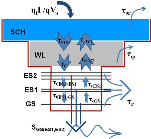
Figure 1. Schematic diagram of the components in the InAs/ GaAs QD lasers for the conduction band; The levels are related to: separate confinement heterostructures (SCH), wetting layer (WL), second excited state (ES2), first excited state (ES1) and the ground state (GS) of a QD.
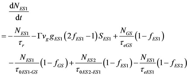
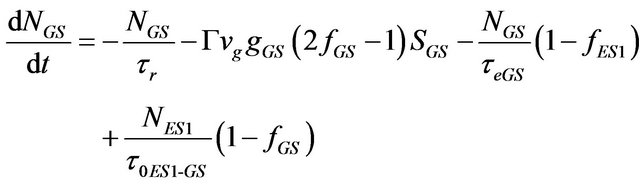
of the carriers decay (τqr), and WL obtains few carriers which are escaped back from ES2 (τeES2). Processes occur for carriers in the GS, ES1 and ES2 are in the same way. Thus, ES1 is only considered for demonstration. Parts of the carriers come to the ES1 from ES2 via relaxation (τ0ES2-ES1) and parts of the carriers relax from ES1 to GS (τ0ES1-GS). Also, some carriers which are escaped from the GS, go to the ES1 (τeGS) and on the other side some of its carriers escape to the ES2 (τeES1). Some parts of the carriers perform decay due to the effect of spontaneous and Auger effects (τr). The remaining carriers contribute in the stimulated emission to produce laser photons. Based on analysis of carrier dynamics for a QD, the rate equations for the density of carrier (electrons) and photons (photon populations) are given in Equations (1)-(8) respectively:
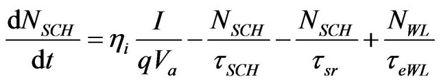 (1)
(1)
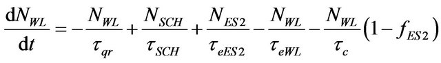 (2)
(2)
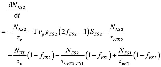 (3)
(3)
 (4)
(4)
 (5)
(5)
 (6)
(6)
 (7)
(7)
 (8)
(8)
where, in the excitonic model which is assumed that the number of electrons and holes are equal, parameters NSCH, NWL, NES2, NES1, and NGS show the density of carriers in the SCH, WL, ES2, ES1 and GS respectively. In addition, SGS, SES1 and SES2 are the density of photons in the GS, ES1 and ES2 level respectively. Quantity ηi is coefficient of injected current rate (I, injected current), and q is unit charge; Volume of active region is defined by Va. The terms ,
,  ,
,  ,
,  , and
, and  represent decay rates of carrier density in SCH, WL, ES2, ES1, and GS respectively. The terms with form
 , show the carrier escape rate from the current level to higher level, while τe is the carrier escape time. Moreover,
  and
and , are carrier relaxation rate from higher into current level and from current level into the lower one respectively. The τ0, is the relevant carrier relaxation time. Parameter f indicates occupation probability of destination level, which will be defined later on. Also,
  is carrier relaxation rate from the WL to ES2, which τc shows carrier relaxation time. Plus,
  ,
,  and
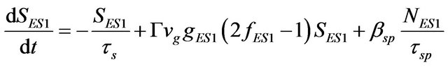
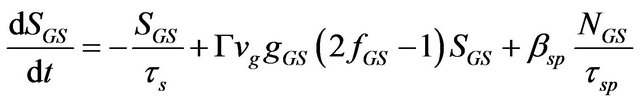
and  are corresponding to photon decay rates, with τs as photon lifetime. Terms
 ,
,  and
and  define photon generation rate by spontaneous recombination, where βsp is spontaneous emission coupling factor, and τsp is spontaneous recombination time. Finally,
  ,
,  and
and  represent photon generation rate (+) and carrier recombination rate (−) due to stimulated emission, where Γ is the optical confinement factor, vg is the group velocity, and g is the peak gain of material.
The Pauli’s exclusion principle controls transition of carriers from one level to another one (with f as occupation probability, ). So fGS, fES1 and fES2 represent occupation probabilities of GS, ES1 and ES2 respectively by carrier, where N is carrier density in current state, ND is the total number of QDs. Defining μ as degeneracy, the μGS, μES1 and μES2 are degeneracies of GS, ES1 and ES2 respectively; and the corresponding values are 2, 4 and 6.
3. Simulations Results
There are eight variables in the equations 1 - 8 that can be calculated numerically using 4th order Runge-Kutta method. Using analysis of the carrier dynamics and photon densities of individual levels, we are able to investigate relaxation oscillations, laser response to step injection current, P-I characteristic curve, relation between carrier relaxation time into the ground state and the laser switch-on, and achievable output power. The computational results are presented in the following sections.
3.1. Carrier Dynamics
To describe the dynamic behavior of the photon and carrier density in the three levels of QD and their variation due to increasing injection current, the relaxation time τc, τ0ES2-ES1 and τ0ES1-GS, can be taken 25, 25 and 75 ps respectively, for the considered QD laser in this paper. Since each energy level has a different threshold current which increases from the GS to the ES2 level systematically, the relevant densities were calculated and plotted for currents near and above threshold. For the GS, photon and carrier density, and for the excited levels, only the photon densities were plotted and are shown in the Figures 2(a)-(d).
As it can be seen in the Figures 2(a)-(d), the carrier and photon densities for different levels reach steady states after viewing relaxation oscillations at the early stages of injection current. The relaxation oscillations represent interaction between GS, ES1 and ES2 energy levels occupation and generation of carriers and photons in the cavity. Thus, it is consequence of involving the carriers’ dynamics inside quantum dots. At current values below the threshold, there is no oscillation, and photon densities of each level are very small. As injection current increases, photon density would increase and the QD lasing begins. The increasing will continue until the density reaches a constant value and then further injection increasing does not change the photon density.
3.2. Laser Response to a Step Injection Current
The relationship between the laser output power and photon density is as follows:
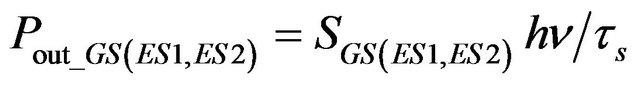 (9)
(9)
where, hν is the energy of each photon, and τs is photon lifetime in the cavity which can be obtained from:
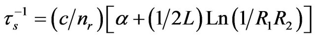 (10)
(10)
In this equation, nr is the refractive index of medium, α is the total loss of the laser which consists of two parts: the internal loss (e.g. αi = 2 cm−1) and mirror loss (e.g. αm = 12 cm−1). Parameters R1 and R2 are reflectivity of mirrors, and L is the length of the active medium.
We can investigate lasers’ response and its time variations due to the current injection change, the laser switchon time and achievable output power. The switch-on time (τswitch-on) is the duration when the output power reaches half the maximum value of the first peak.
In the Figure 3(a) output power versus time for the GS is depicted when injected current was 12 mA. Calculation shows the switch-on time value is 2.3 ns, and the laser reaches steady state after about 4.5 ns following some fluctuations. Variation of output power for the GS by increasing injected current is shown in the Figure 3(b).

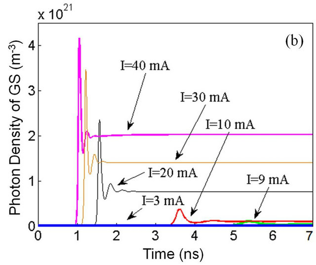
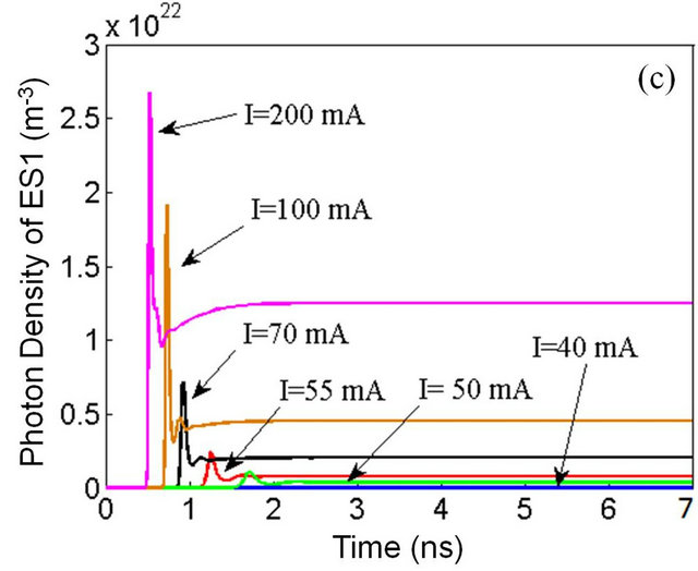

Figure 2. (a) Plot of carrier density in the GS; photon density for the (b) GS, (c) ES1 and (d) ES2 for different currents.
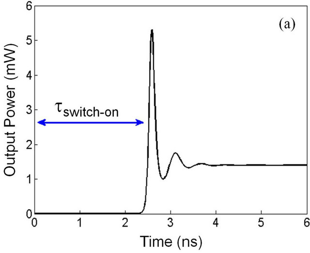
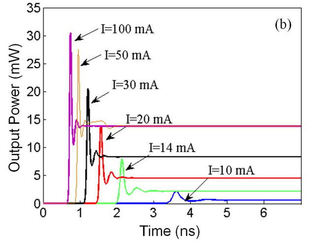
Figure 3. Laser output power vs. time, for the GS (a) with injected current 12 mA; (b) Different injection currents.
As it can be seen from the graph, the switch-on and stability times decrease with increasing injection current and the power’s peak and the achieved steady power of the laser would increase. At currents exceed 50 mW, the laser is saturated, and therefore by further increasing of the input current, laser’s stabilized power remains unchanged, but the turn-on time continues to its decreasing.
3.3. Characteristic Curve (P-I)
One of the most practical laser characteristics is the P-I curve. The P-I characteristic curve could be sketched by computing the laser output power for chosen different values of injection current in the laser active medium.
Threshold current and slope efficiency, dP/dI, can be obtained using this curve. Normally, below the threshold injection current, the output light intensity is negligibly small, and above threshold, the output power of laser shows linearly increasing behavior. The P-I curve for the GS is shown in the Figure 4(a), which indicates that the threshold current is ~9 mA. Also, computed value for the slope efficiency is 0.4 W/A that means 1 mA further increasing in the injected current is needed to have 0.4 mW power increasing. The Figure 4(b) shows the P-I curve for the three energy states. It is assumed that the energy of emitted photon is the same for all the three levels. As mentioned earlier, to excite carriers to higher energy levels, the injection current is needed to be increased. Therefore, the threshold current is higher for the upper energy levels.
As it can be seen in the Figure 4(b), by starting the current injection, carriers of GS begin to emit photons. While the GS related emission output is saturated, ES1 carriers will begin to emit photons. Likewise, as the ES1output is saturated, photon emission from the ES2 will be started. The calculated threshold current for the GS, ES1 and ES2 are 9, 45 and 238 mA respectively.
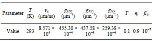
It should be mentioned that the laser must not end up to failure due to very high injected current. Some parameters which have been used in this study to simulate QD lasers are shown in the Tables 1 and 2.
4. Conclusion
In this paper, InAs/GaAs QD Laser were modeled and simulated based on a set of eight coupled rate equations for the carrier and photon densities in five energy levels, including SCH, WL, ES2, ES1 and GS. The rate equations were solved using 4th order Runge-Kutta method using MATLAB software. Time variation of the carrier and
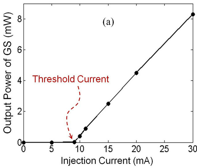
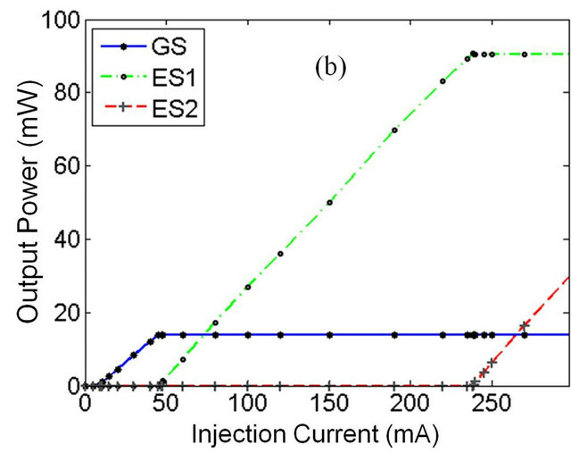
Figure 4. (a) The P-I curve for GS lasing which shows threshold current is 9 mA, and slope efficiency dP/dI = 0.4 W/A; (b) The P-I curve related to the GS, ES1 and ES2.
Table 1. Parameters used in the simulation.
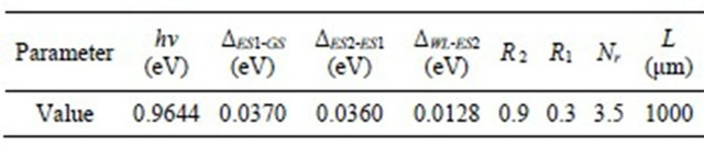
Table 2. Other parameters used in the simulation.
photon densities, laser’s response to various step current injections, and P-I characteristic curve for the three energy levels ES2, ES1 and GS, were investigated. The results have shown that by increasing the injection current, the photons density of each level increases till the laser system is saturated. Also, it has been found that the QD lasers have lower threshold currents in comparison with the conventional lasers. It was also seen that by increasing injection current, switch-on time and stabilized time of laser would decrease, while peak power and stabilized power increase. The power increase would exist until photons emissions at each level reach steady state. Subsequent to stabilization of emission power in each level, the upper level will start to emit photons, and contributes in the output of the device.
REFERENCES
- M. Asada, Y. Miyamoto and Y. Suematsu, “Gain and the Threshold of Three-Dimensional Quantum-Box Lasers,” IEEE Journal of Quantum Electronics, Vol. 22, No. 9, 1986, pp. 1915-1921. doi:10.1109/JQE.1986.1073149
- N. N. Ledentsov, V. M. Ustinov, A. Yu. Egorov, A. E. Zhukov, M. V. Maximov, I. G. Tabatadze, P. S. Kop’ev, “Optical Properties of Heterostructures with InGaAsGaAs Quantum Clusters,” Semiconductors, Vol. 28, No. 8, 1994, pp. 832-834.
- J. A. Timpson, et al., “Single Photon Sources Based upon Single Quantum Dots in Semiconductor Microcavity Pillars,” Special Issue of the Journal of Modern Optics, Vol. 54, No. 2-3, 2007, pp. 453-465. doi:10.1080/09500340600785055
- S. Reitzenstein et al., “Electrically Driven Quantum Dot Micropillar Light Sources,” IEEE Journal of Selected Topics in Quantum Electronics, Vol. 17, No. 6, 2011, pp. 1670 - 1680. doi:10.1109/JSTQE.2011.2107504
- W. T. Silfvast, “Laser Fundamentals,” 2nd Edition, Cambridge University Press, Cambridge, 2004.
- O. Svelto, “Principles of Lasers,” 5th Edition, Springer Science + Business Media, LLC., New York, 2010.
- S.-F. Lv, I. Montrosset, M. Gioannini, S.-Z. Song and J.-W. Ma, “Modeling and Simulation of InAs/GaAs Quantum Dot Lasers,” Optoelectronics Letters, Vol. 7, No. 2, 2011, pp. 122-125. doi:10.1007/s11801-011-0102-3
- G. A. P. Thé, “How to Simulate a Semiconductor Quantum Dot Laser: General Description,” Revista Brasileira de Ensino de Fisica, Vol. 31, No. 2, 2009, p. 2302.