J. Biomedical Science and Engineering, 2010, 3, 488-495
doi:10.4236/jbise.2010.35068 Published Online May 2010 (http://www.SciRP.org/journal/jbise/
JBiSE
).
Published Online May 2010 in SciRes. http://www.scirp.org/journal/jbise
A consistency contribution based bayesian network model for
medical diagnosis
Yan-Ping Yang
School of Computer Science and Technology, Huazhong University of Science and Technology, Wuhan, China.
Received 8 February 2010; revised 1 March 2010; accepted 5 March 2010.
ABSTRACT
This paper presents an effective Bayesian network
model for medical diagnosis. The proposed approach
consists of two stages. In the first stage, a novel fea-
ture selection algorithm with consideration of feature
interaction is used to get an undirected network to
construct the skeleton of BN as small as possible. In
the second stage for greedy search, several methods
are integrated together to enhance searching per-
formance by either pruning search space or over-
coming the optima of search algorithm. In the ex-
periments, six disease datasets from UCI machine
learning database were chosen and six off-the-shelf
classification algorithms were used for comparison.
The result showed that the proposed approach has
better classification accuracy and AUC. The pro-
posed method was also applied in a real world case
for hypertension prediction. And it presented good
capability of finding high risk factors for hyperten-
sion, which is useful for the prevention and treatment
of hypertension. Compared with other methods, the
proposed method has the better performance.
Keywords: Bayesian Network; Medical Diagnosis;
Feature Selection; Greedy Search
1. INTRODUCTION
Machine learning classification techniques have been
applied to medical diagnosis tasks [1-4]. With many ad-
vantages over other methods, Bayesian network has be-
come a promising tool in medical diagnosis [5-9]. It can
reason under uncertainty by providing a concise repre-
sentation of a joint probability distribution over a set of
random variables [6,10]. Due to its graphical representa-
tion, a Bayesian network is easily understandable [11].
In addition, the diagnostic performance with Bayesian
networks is often surprisingly insensitive to imprecision
in numerical probabilities [12].
Bayesian network based diagnosis requires the lear-
ning of the Bayesian network structure, which is an op-
timization problem in the search space of the DAGs (di-
rected acyclic graph). In general, researchers treat this
problem in two distinctly different ways: the constraint-
based method [13] and the search-and-scoring method
[14,15]. The constraint-based methods are computation-
ally effective. However, the search-and- scoring methods
may produce more accurate results than the constraint-
based methods [15]. In addition, constraint-based meth-
ods may fail to provide orientations for all edges in a
network [13]. In this work we focus on structure learning
and consider search-and-scoring methods.
When learning the structure of a Bayesian network
model, however, search-and-scoring methods still face
great challenges [16], because the true structure may not
be identified by a finite number of observations, and it
may be computationally intractable when the number of
possible network structures grows super exponentially.
To prune the search space, the existing methods depend
on either setting a uniform bound on the number of par-
ents [17], or conditional dependency test [18], which
may degrade the performance of classification. As for
the computation efficiency, hill-climbing search algo-
rithm is the most commonly used because of its good
trade-off between accuracy of the obtained model and
ease of implementation. However, the well-known prob-
lem, myopia, may hinder the algorithm from finding the
global optima.
In this paper, a new Consistency-Contribution based
Bayesian Network algorithm, named CCBN, is proposed
for medical diagnosis. To build the skeleton of Bayesian
network, a novel feature selection method with the con-
sideration of feature interaction is used to efficiently
construct an undirected network. Further more, to en-
hance the performance of search algorithm, “AND” or
“OR” strategy [19] is used to prune search space, while
random start, beam-search and look-ahead help to over-
come the optima of hill-climbing algorithm. To evaluate
the effectiveness of the proposed algorithm in various
medical problems, six disease datasets from the UCI
machine learning repository were selected, and six off-
the-shelf classifiers were used for comparison. Moreover,

Y. P. Yang / J. Biomedical Science and Engineering 3 (2010) 488-495 489
a real world application on hypertension dataset was
chosen to present its capability of finding high risk fac-
tors for hypertension. Its classification performance was
further evaluated against other algorithms.
The rest of this paper is organized as follows. Section
2 introduces the necessary preliminaries about Bayesian
network. In Section 3, the proposed classifier is de-
scribed in detail. Then experiments on six disease data-
sets from the UCI machine learning repository are pre-
sented in Section 4. Later in Section 5, the proposed
method is applied in a real world case for hypertension
prediction to further evaluate its performance. Conse-
quently in Section 6, the main contribution of this paper
is summarized.
2. PRELIMINARIES
2.1. Bayesian Network
A Bayesian network B = (G, Θ) consists of two parts [7].
The first part is a network structure, which is a directed
acyclic graph (DAG) G with each variable repre-
sented as a node. The edges in the DAG represent statis-
tical dependencies between the variables. The second
part, Θ, is a set of parameters describing the probability
density.
i
X
The problem of learning a BN can be stated as follows:
given a finite data set of instances
of variable X, find a minima set Ф to construct a graph
structure G with proper parameters Θ that best matches
D. In the commonly used search-and-scoring methods, a
scoring function is usually used to evaluate how well the
DAG G explains the data and then to search for the best
DAG that optimizes the scoring function. In our pro-
posed algorithm, Bayesian scoring criterion [14] is cho-
sen. It computes the posteriori probability of a network
given the data and prior knowledge [20].
},,{ 21 n XXXD 
2.2. Feature Selection
To get the skeleton of a BN, Ф, is a solution to feature
selection [21]. In real-world classification problems,
feature selection is indispensable to identify the most
useful relevant features from data, and remove the
irrelevant and redundant features [22]. Here, we define
the feature relevant as that in [14]: in a feature set F, a
feature is relevant to a class C if and only if there ex-
ists a subset , for which
i
F
}{ i FFS  )S,FC(P i)SC(P;
otherwise is irelevant.
i
F
To find the relevant features, many effective algo-
rithms have been developed [23,24], but they most
often assume that features are independent. Due to
attribute interaction [25], however, there are many
features that can be considered as irrelevant when
evaluated independently; but when they are combined
with other features, their relevancy may be significant.
Thus, unintentional removal of these features could
lead to poor classification performance because of the
loss of useful information.
Jakulin and Bratko [26,27] attempted to address this
issue, but their methods can only deal with low order
interaction. Later, Zhen Zhao [28] presented a more
efficient algorithm by searching for interacting fea-
tures. In this paper, we will use consistency measure to
construct the skeleton of BN with consideration of
feature interaction.
3. METHOD
3.1. Overview
In this section, we present our consistency measure
based Bayesian Network algorithm, named CCBN. The
algorithm is a two-step process: Firstly, an undirected
network is constructed as the prototype of a BN’s skele-
ton Ф based on symmetrical uncertainty and consis-
tency hypothesis. This process finds a set that is as small
as possible, but can deal with feature interactions in
variable selection, and contain all parents, children and
co-parents (attribute interaction) of each variable. In the
second step, several methods are integrated together to
enhance the performance of search algorithm by re-
stricting the search space and overcoming the myopia of
Hill-climbing search.
3.2. Constructing the Skeleton of BN
To construct the skeleton of a BN, an undirected network
will be discovered in two phases. In phase-one, all vari-
ables (features) are ranked with regard to their SU (sym-
metrical uncertainty) and stored in the candidate set PC
in descending order. In the second phase, the backward
phase, features with less consistency-contribution will be
removed from the candidate set PC. This elimination
process is based on the consistency measure and takes
into account feature interaction when removing both
irrelevant and redundant features. In the end, the undi-
rected network is obtained with candidate set PC. It will
be used as the skeleton of BN.
As a fast correlation measure [24], SU is based on
mutual information to measure the common information
shared by two variables. It attempts to increase the
chance for a strongly relevant feature to remain in the
selected subset. The SU between the class label C and a
feature is formulated as:
i
F







)()(
)(
2)(CHFH
C,FM
C,FSU
i
i
i (1)
where H(Fi) and H(C) are the marginal entropies, and
M(Fi,C) is the joint entropy.
This formula compensates for information gain’s bias
toward features with more values and normalizes its
values to the range [0,1] with the value 1 indicating that

490 Y. P. Yang / J. Biomedical Science and Engineering 3 (2010) 488-495
knowledge of the value of the feature Fi can completely
predict the value of class label C and the value 0 indi-
cating that the feature Fi and class label C is independ-
ent.
After all features are ranked in descending order with
regard to their SU values, a backward elimination me-
thod will be performed. However, in our method, SU
will not be the criterion for elimination, because it can’t
guarantee that the interacting features are ranked highly.
Instead, a novel consistency measure with the consi-
deration of feature interaction is used to remove both
irrelevant and redundant features.
In a dataset , there is inconsistency
if at least two instances have the same value for a feature
space , but they are categorized into
different classes. Those inconsistent instances will be
grouped together into a subset , named as inconsis-
tent instance set. Every has its inconsistency count
},,{ 21 m dddD 
},, 2n FF 
D
i
D
{1 FF 
()
i
F
i
D IC . Let 12 ,,
p
 DD D represents all inconsistent
instance sets of D, the inconsistency rate of D is:
1
()
()
F
i
ip
F
IC
ICR Dm



D
(2)
Here, m represents the number of instances in D.
If i
F
is irrelevant or redundant, removing it from F
will have no effect on the number of inconsistent instant-
ces. Consequently, there will be .
If
{}
() ()
FFFi
ICR DICRD


i
F
is a relevant feature, no matter whether it has
feature interaction or not, its removal will bring more
inconsistent instances,{}
() ()
FFFi
I
CR DICRD

. This
unique character, named as consistency contribution,
makes it a good metric for feature selection by taking the
feature interaction into consideration.
In our method, a feature i
F
’s consistency contribu-
tion is formalized as:
{}
(,)()()
iFF F
i
CC FFICRDICRD

 (3)
From Eq.3, we can conclude that: higher consistency
contribution value means higher relevancy; and the zero
value indicates that it is either irrelevant or redundant
feature. Using certain threshold value δ those weak
relevant feature [16] can also be removed from if PC
()
i
CC F

. It will help to restrict the search space.
Based on the consistency-contribution, the elimination
operation will start from the end of the ranked feature
list. If the consistency-contribution of a feature is less
than a predefined threshold δ (0 < δ < 1), the feature is
considered immaterial and can be removed; otherwise it
is selected. The process is repeated until all features in
the list are checked. A large δ is associated with a high
probability of removing relevant features. δ is assigned
0.0001 in this paper if not otherwise mentioned.
3.3. DAG Search
After an undirected network is constructed as the proto-
type of Ф, a local hill climbing algorithm will be used to
search for the best DAG that optimizes the scoring func-
tion in the restricted space of DAGs.
To make the greedy hill climbing algorithm more effi-
cient, our method takes into account several aspects, like
preprocessing, starting solution, how to acquire neigh-
bors and score metrics for candidate neighbors.
Before performing the hill-climbing algorithm, the
search space of DAGs is initially restricted by using
“OR” or “AND” strategy [19], because of the likely
asymmetric dependencies in the finite sample scenario
(i.e., the edge a-b may be found on a but not on b). In
“OR” strategy, an arc is excluded only if it was not
found in either direction, while “AND” strategy requires
edges to be found in both directions.
In addition, our DAG search will start with a random
start DAG network rather than an empty one (i.e., the
one with no edges). Based on the restricted search space
for DAGs, a random number of edges will be chosen
randomly. The edge will be added to the original DAG
only if it is discovered in the process of constructing the
undirected network.
To obtain the neighbor at each search step, the legal
operators used are arc addition, arc deletion, and arc
reversal. Of course, except in arc deletion, we have to
make sure that there is no directed cycle introduced in
the graph. For fast evaluation of candidate sub-graphs
(neighbors), the Bayesian scoring criterion is used in our
work.
To overcome the myopia of hill climbing algorithm,
the 2-step look ahead in good directions (LAGD) hill
climbing is used. Further more, 5 best evaluation op-
erations will be considered at each search step.
Following is the procedure of our DAG searching:
1) Restrict search space of DAG with “OR” or
“AND” strategy;
2) Form an original DAG Mc with random starting
and get the Bayesian scoring metric for Mc;
3) Obtain all neighbors of current candidate DAG Mc
by getting all possible directional orientations for the
edges in Mc and compute the Bayesian scoring metric
for each neighbor;
4) By ranking Bayesian scoring metric for all
neighbors in descending order, store the 5 best valued
network structures in a specific set B1;
5) For each candidate stored in set B1, get its
neighbors in the same way as 3) and get its Bayesian
scoring metric;
6) Choose the neighbor with highest Bayesian scoring
metric in step 5), and mark it as new candidate DAG
Mnew;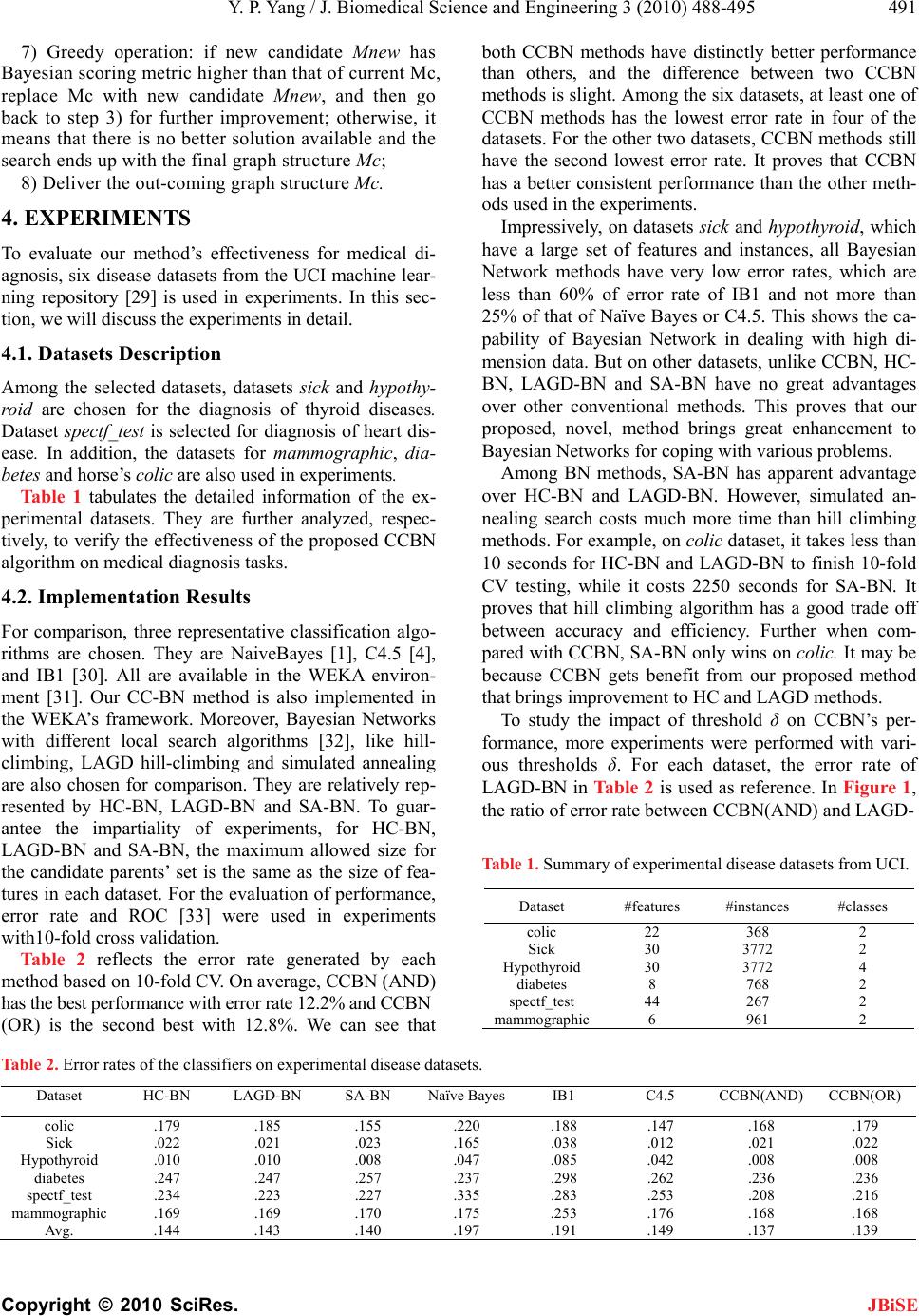

Y. P. Yang / J. Biomedical Science and Engineering 3 (2010) 488-495 491
4. EXPERIMENTS
7) Greedy operation: if new candidate Mnew has
Bayesian scoring metric higher than that of current Mc,
replace Mc with new candidate Mnew, and then go
back to step 3) for further improvement; otherwise, it
means that there is no better solution available and the
search ends up with the final graph structure Mc;
8) Deliver the out-coming graph structure Mc.
To evaluate our method’s effectiveness for medical di-
agnosis, six disease datasets from the UCI machine lear-
ning repository [29] is used in experiments. In this sec-
tion, we will discuss the experiments in detail.
4.1. Datasets Description
Among the selected datasets, datasets sick and hypothy-
roid are chosen for the diagnosis of thyroid diseases.
Dataset spectf_test is selected for diagnosis of heart dis-
ease. In addition, the datasets for mammographic, dia-
betes and horse’s colic are also used in experiments.
Table 1 tabulates the detailed information of the ex-
perimental datasets. They are further analyzed, respec-
tively, to verify the effectiveness of the proposed CCBN
algorithm on medical diagnosis tasks.
4.2. Implementation Results
For comparison, three representative classification algo-
rithms are chosen. They are NaiveBayes [1], C4.5 [4],
and IB1 [30]. All are available in the WEKA environ-
ment [31]. Our CC-BN method is also implemented in
the WEKA’s framework. Moreover, Bayesian Networks
with different local search algorithms [32], like hill-
climbing, LAGD hill-climbing and simulated annealing
are also chosen for comparison. They are relatively rep-
resented by HC-BN, LAGD-BN and SA-BN. To guar-
antee the impartiality of experiments, for HC-BN,
LAGD-BN and SA-BN, the maximum allowed size for
the candidate parents’ set is the same as the size of fea-
tures in each dataset. For the evaluation of performance,
error rate and ROC [33] were used in experiments
with10-fold cross validation.
Table 2 reflects the error rate generated by each
method based on 10-fold CV. On average, CCBN (AND)
has the best performance with error rate 12.2% and CCBN
(OR) is the second best with 12.8%. We can see that
both CCBN methods have distinctly better performance
than others, and the difference between two CCBN
methods is slight. Among the six datasets, at least one of
CCBN methods has the lowest error rate in four of the
datasets. For the other two datasets, CCBN methods still
have the second lowest error rate. It proves that CCBN
has a better consistent performance than the other meth-
ods used in the experiments.
Impressively, on datasets sick and hypothyroid, which
have a large set of features and instances, all Bayesian
Network methods have very low error rates, which are
less than 60% of error rate of IB1 and not more than
25% of that of Naïve Bayes or C4.5. This shows the ca-
pability of Bayesian Network in dealing with high di-
mension data. But on other datasets, unlike CCBN, HC-
BN, LAGD-BN and SA-BN have no great advantages
over other conventional methods. This proves that our
proposed, novel, method brings great enhancement to
Bayesian Networks for coping with various problems.
Among BN methods, SA-BN has apparent advantage
over HC-BN and LAGD-BN. However, simulated an-
nealing search costs much more time than hill climbing
methods. For example, on colic dataset, it takes less than
10 seconds for HC-BN and LAGD-BN to finish 10-fold
CV testing, while it costs 2250 seconds for SA-BN. It
proves that hill climbing algorithm has a good trade off
between accuracy and efficiency. Further when com-
pared with CCBN, SA-BN only wins on colic. It may be
because CCBN gets benefit from our proposed method
that brings improvement to HC and LAGD methods.
To study the impact of threshold δ on CCBN’s per-
formance, more experiments were performed with vari-
ous thresholds δ. For each dataset, the error rate of
LAGD-BN in Table 2 is used as reference. In Figure 1,
the ratio of error rate between CCBN(AND) and LAGD-
Table 1. Summary of experimental disease datasets from UCI.
Dataset #features #instances #classes
colic 22 368 2
Sick 30 3772 2
Hypothyroid 30 3772 4
diabetes 8 768 2
spectf_test 44 267 2
mammographic6 961 2
Table 2. Error rates of the classifiers on experimental disease datasets.
Dataset HC-BN LAGD-BN SA-BN Naïve BayesIB1 C4.5 CCBN(AND) CCBN(OR)
colic .179 .185 .155 .220 .188 .147 .168 .179
Sick .022 .021 .023 .165 .038 .012 .021 .022
Hypothyroid .010 .010 .008 .047 .085 .042 .008 .008
diabetes .247 .247 .257 .237 .298 .262 .236 .236
spectf_test .234 .223 .227 .335 .283 .253 .208 .216
mammographic .169 .169 .170 .175 .253 .176 .168 .168
Avg. .144 .143 .140 .197 .191 .149 .137 .139

492 Y. P. Yang / J. Biomedical Science and Engineering 3 (2010) 488-495
BN is shown to reflect the effect of threshold δ. meaning of the threshold, for example, from a statis-
tical aspect, is another interesting topic for future work.
It is likely that this turning point may not be independent
of the dataset (problem) to be analyzed. If it is true, we
hope to propose some feasible approaches that could
tune the threshold automatically for a specific problem.
Figure 1 shows that on hypothyroid, colic, diabetes
and mammographic, CCBN is better than that of
LAGD-BN, even for δ = 0. Such an improvement should
owe to random start which has depressed local subop-
tima. Also, with δ = 0.00001 or δ = 0.0001, CCBN
shows much more improvement over LAGD-BN for all
datasets except sick. This supports our claim that our
method is much more efficient for feature selection due
to the consideration of feature interaction. However, it
should be noted that CCBN’s advantage over LAGD-BN
is not consistent. On hypothyroid, CCBN’s performance
is worse than LAGD-BN’s when δ = 0.01. On sick,
CCBN has no win. We will discuss about this more in
next section.
5. APPLICATION ON HYPERTENSION
PROBLEM
In this section, a real-case from medical diagnosis is pre-
sented. We will show that our proposed method is capa-
ble of finding the high risk factors for hypertension di-
agnosis and prediction. Also, classification result on hy-
pertension is evaluated against other algorithms.
5.1. Problem Description
Also, when studying the impact of δ on CCBN’s per-
formance, we found that for δ with range from 0 to 0.001,
the change of error rate for each dataset is less than 10%.
This means that our method is insensitive to the thresh-
old value δ. This improvement may benefit from random
start.
As one of the most common disease in the world, hyper-
tension is considered to be present when a person’s
systolic/diastolic blood pressure is consistently 140/
90 mmHg or greater [34]. It is affecting estimated 600
million people worldwide [35], and that number is ex-
pected to increase to 1.56 billion by 2025 [36]. There-
fore, it is meaningful to develop a computer-aid system
for its diagnosis and prediction.
Although classification accuracy is our focus, ROC is
also introduced in our experiment’s evaluation. Accord-
ing to Table 3, CCBN method has highest average area
under ROC (AUR). Although its AUR is not highest on
colic, spectf-test and diabetes, the difference is slight.
Also, it is apparent that BN methods have higher AUR
than other traditional methods.
In our experiments, the data from the hypertension
study were specifically collected by Hubei Provincial
Center for Disease Control and Prevention in China. The
investigation was conducted in compliance with the IRB
4.3. DISCUSSION
By comparing CCBN with other classification algori-
thms, experiments proved that CCBN can achieve better
performance, but there are still some issues that should
be addressed for improvement.
First, the error rate of CCBN (AND) on four of six
datasets, is better than that of the other methods used in
our experiments. On colic and mammogrpahic, however,
this does not hold, although CCBN (AND) is still the
second best. This suggests that there may be some properties
Second, although on most dataset CCBN proves to be
insensitive to threshold value, threshold value still shows
big impact on spectf-test. Also, the best error rate for
different datasets happens on different thresholds. It is
obvious that the ideal choice of a threshold is the turning
point that provides the lowest error rate. Exploring the
Figure 1. The ratio of error rate between CCBN (AND) and
LAGD for different thresholds on six UCI datasets.
Table 3. AUR of the classifiers on experimental disease datasets.
Dataset HC-BN LAGD-BN SA-BN Naïve BayesIB1 C4.5 CCBN(AND) CCBN(OR)
colic .874 .873 .890 .842 .795 .813 .88 .876
Sick .958 .959 .960 .925 .804 .951 .965 .964
Hypothyroid .482 .483 .519 .282 .500 .197 .703 .703
diabetes .807 .807 .800 .819 .662 .751 .799 .799
spectf_test .765 .772 .799 .849 .620 .592 .795 .746
mammographic .897 .897 .897 .894 .744 .855 .898 .898
Average .797 .798 .810 .768 .688 .693 .840 .831
JBiSE

Y. P. Yang / J. Biomedical Science and Engineering 3 (2010) 488-495 493
approved study protocol and the law in China. It in-
cluded a representative sample of 3053 adults: 1438
males, 1610 females and five without sex information.
The participants ranged in age from 35 to 92 years old
and average age was 51 years old. The prevalence of
hypertension was 26.9%. The 155 features in the data-
base include sample population characteristics, heal- th,
health care, habits of life, and etc. Obviously irrelevant
and sparse (more than 50% missing data) features were
discarded from further investigation. The features used
in the experiments were recommended by the clinician
for diagnosis. The resulting dataset contained 32 poten-
tial risk factors such as age, waistline, body-mass index
(BMI) and etc (detailed information about some impor-
tant attributes are presented in Table 4).
5.2. Classification Results
In order to assess the effectiveness of the proposed ap-
proach, its performance was evaluated against that of
some off-the-shelf algorithms. The performance of the
different algorithms is listed in Table 5, which contains
Error rate, Sensitivity (SN), Specificity (SP), Positive
predictive value (PPV), and Negative predictive value
(NPV). The result shows that CCBN with ‘AND’ strat-
egy has the same performance as that with “OR” strat-
egy for hypertension classification. Both CCBNs have
the lowest error rate on the hypertension classification.
Besides error rate, CCBN methods also have the best
specificity, PPV and AUR. On sensitivity, although Na-
ive Bayes has a slightly better performance than CCBNs,
the difference is not significant. Therefore, we can con-
clude that CCBN has better performance on hyperten-
sion classification than other methods.
5.3. Risk Factor Analysis
For the prediction of hypertension, CCBN tried to find
those likely high risk factors. These high risk factors
enabled the classifiers to achieve their best performance
and also would give us important guide to hypertension
prevention and treatment.
In experiment, CCBN marked age, BMI and blood
pressure as the high risk factors in hypertension deve-
lopment. This result is consistent with many clinical
studies.
As we know, lifestyle plays an important role in the
development and treatment of hypertension. For the die-
tary intake, fish, meat, soybean products, eggs and diary
are selected by CCBN, which is coherent with current
knowledge about hypertension. According to exercise,
the original data have three attributes: frequency of ex-
ercise in a week, taking exercise every day or not, num-
ber of days in a week that have more then 30 minutes
spent on exercise. In CCBN, the first two attributes are
ignored, because the third attribute has more or at least
not less information about the impact of exercise on hy-
pertension than other two attributes.
Among the attributes about social background, na-
tionality and occupation are removed from BN. Remar-
kably education background and marital status are also
selected as key factors in prediction of hypertension.
CCBN shows that higher education will lead to less risk
of hypertension, and the single is more susceptible to
hypertension than the married. It is reasonable because
people with higher education are more aware of the jeo-
pardy of hypertension and have more knowledge about
the prevention of hypertension, which in turn leads to
good lifestyle. Similarly for marital status, the married is
more likely to lead regular lifestyle and have more hea-
lthy diet than the single.
6. CONCLUSIONS
Bayesian network is a powerful learning technique to
tackle the uncertainty in medical problems, but learning
Table 4. Summaries of mean and standard deviations of some
important features in hypertension dataset.
Features Mean S.D Missing (%)
age 51.43 12.32 0.00
sex 1.53 0.50 0.00
cigarette smoker 1.63 0.49 0.04
Grossincome families 3.65 1.19 0.01
excessive alcohol intake 1.69 0.46 0.07
body mass index (BMI) 22.14 3.03 0.03
family history of hypertension 1.12 0.33 0.10
physical inactivity 1.98 1.25 0.08
marital status 1.24 0.71 0.01
education 2.35 0.87 0.00
Table 5. Performance of classifiers for the hypertension dataset based on 10-fold CV.
Algorithms Error rate Sensitivity Specificity PPV NPV
CCBN(AND) .163 .553 .942 .779 .851
CCBN(OR) .163 .553 .942 .779 .851
NaïveBayes .198 .555 .892 .656 .845
C4.5 .186 .520 .922 .711 .839
IB1 .329 .309 .805 .369 .759
HC-BN .164 .553 .940 .772 .851
SA-BN .164 .550 .942 .777 .850
LAGD-BN .164 .555 .941 .776 .852

494 Y. P. Yang / J. Biomedical Science and Engineering 3 (2010) 488-495
its structure is a great challenge, which may hinder its
wide application in medicine. In this paper, the CCBN
algorithm is proposed for medical diagnosis. Our method
firstly constructs the skeleton of BN with consideration
of feature interaction, and then performs the efficient
search for an optimal BN network. Case studies on dis-
ease datasets and application on hypertension predict-
tion show that the proposed method is a promising tool
for computer-aided medical decision system, because it
has better classification accuracy and consistency than
other traditional methods.
REFERENCES
[1] Mitchell, T.M. (1997) Machine learning. McGraw-Hill,
New York.
[2] Jordan, M.I. (1995) Why the logistic function? A tutorial
discussion on probabilities and neural networks techno-
logy. MIT Computational Cognitive Science Report 9503,
Massachusetts.
[3] Aha, D., Kibler, D. and Albert, M. (1991) Instance-based
learning algorithms. Machine Learning, 6(1), 37-66.
[4] Quinlan, J.R. (1993) Programs for machine learning. San
Mateo, Morgan Kaufmann, California.
[5] Lisboa, P.J.G., Ifeachor, E.C. and Szczepaniak, P.S. (2000)
Artificial neural networks in biomedicine. Springer-Ver-
lag, London.
[6] Cooper, G.F. and Herskovits, E. (1992) A Bayesian me-
thod for the induction of probabilistic networks from data.
Machine Learning, 9(4), 309-347.
[7] Lucas, P. (2001) Bayesian networks in medicine: A
model-based approach to medical decision making. Pro-
ceedings of the EUNITE Workshop on Intelligent Systems
in Patient Care, Vienna, 73-97.
[8] Antal, P., Verrelst, H., Timmerman, D., Van Huffel, S.,
De Moor, B., Vergote, I. and Moreau, Y. (2000) Bayesian
networks in ovarian cancer diagnosis: Potentials and
limitations. 13th IEEE Symposium on Computer-Based
Medical Systems, Texas Medical Center, Houston, 103-
108.
[9] van Gerven, M., Jurgelenaite, R., Taal, R., Heskes, T. and
Lucas, P. (2007) Predicting carcinoid heart disease with
the noisy-threshold classifier. Artificial Intelligence in
Medicine, 40(1), 45-55.
[10] Pearl, J. (1988) Probabilistic reasoning in intelligent
systems: Networks of plausible inference. 2nd Edition,
Morgan Kaufmann, San Francisco.
[11] Spirtes, P., Glymour, C. and Scheines, R. (2000) Causa-
tion, prediction, and search. 2nd Edition, the MIT Press,
Cambridge.
[12] Pradhan, M., Henrion, M., Provan, G., Favero, B.D. and
Huang, K. (1996) The sensitivity of belief networks to
imprecise probabilities: An experimental investigation.
The Artificial Intelligence Journal, 85(1-2), 363-397.
[13] Cheng, J., et al. (2002) Learning Bayesian networks from
data: An information theory based approach. The Artifi-
cial Intelligence Journal, 137(1-2), 43-90.
[14] Cooper, G. and Herskovits, E. (1992) A Bayesian method
for the induction of probabilistic networks form data.
Machine Learning, 9(4), 309-347.
[15] Heckerman, D. (1998) A tutorial on learning with Bayes-
ian networks, learning in graphical models. Kluwer Aca-
demic Publishers, Dordrecht, 301-354.
[16] Chickering, D. (1996) Learning Bayesian networks is
NP-complete. In: Fisher, D. and Lenz, H., Eds., Learning
from Data: Artificial Intelligence and Statistics, 4(1)
121-130.
[17] Friedman, N., Nachman, I. and Peer, D. (1999) Learning
Bayesian network structure from massive datasets: The
‘sparse candidate’ algorithm. Uncertainty in Artificial
Intelligence, 15(3), 206-215.
[18] Tsamardinos, I., Brown, L. and Aliferis, C. (2006) The
max-min hill-climbing Bayesian network structure learn-
ing algorithm. Machine Learning, 65(1), 31-78.
[19] Meinshausen, N. and Buhlmann, P. (2006) High dimen-
sional graphs and variable selection with the lasso. The
Annals of Statistics, 34(3), 1436-1462.
[20] Heckerman, D., Geiger, D. and Chickering, D. (1995)
“Learning Bayesian networks: The combination of
knowledge and statistical data. Machine Learning, 20(3),
197-243.
[21] Tsamardinos, I. and Aliferis, C. (2003) Towards prince-
pled feature selection: Relevancy, filters and wrappers.
The 9th International Workshop on Artificial Intelligence
and Statistics, Florida, 334-342.
[22] Guyon, I. and Elisseeff, A. (2003) An introduction to
variable and feature selection. Journal of Machine Lear-
ning Research, 3(7-8), 1157-1182.
[23] Dash, M. and Liu, H. (2003) Consistency-based search in
feature selection. Artificial Intelligence, 151(1-2), 155-
176.
[24] Hall, M. (1999) Correlation based feature selection for
machine learning. Ph.D. Dissertation, University of Wai-
kato, New Zealand.
[25] Kononenko, I. (1994) Estimating attributes: Analysis and
extension of RELIEF. European Conference on Machine
Learning, Catania, 171-182.
[26] Jakulin, A. and Bratko, I. (2003) Analyzing attribute
dependencies. PKDD, Ljubljana.
[27] Jakulin, A. and Bratko, I. (2004) Testing the signifi-
cance of attributes interactions. International Conference
on Machine Learning, 20, 69-73.
[28] Zhao, Z. and Liu, H. (2007) Searching for interacting
features. Proceedings of International Joint Conference
on Artificial Intelligence, Nagoya.
[29] Blake, C., Keogh, E. and Merz, C.J. (1998) UCI reposi-
tory of machine learning databases. University of Cali-
fornia, Irvine. http://www.ics.uci.edu/~mlearn/MLRepo
sitory.html
[30] Aha, D.W., Kibler, D. and Albert, M.K. (1991) Instance-
based learning algorithms. Machine Learning, 6(1),
37-66.
[31] Witten, I.H. and Frank, E. (2005) Data mining-pracitcal
machine learning tools and techniques with JAVA im-
plementations. 2nd Edition, Morgan Kaufmann Publi-
shers, California.

Y. P. Yang / J. Biomedical Science and Engineering 3 (2010) 488-495 495
[32] Bouckaert, R.R. (2008) Bayesian network classifiers in
weka for version 3-5-7. Artificial Intelligence Tools,
11(3), 369-387
[33] Cortes, C. and Mohri, M. (2003) AUC optimization vs.
error rate Minimization. Advances in Neural Information
Processing Systems, 11(10), 356-360.
[34] Chobanian, A.V., Bakris, G.L., Black, H.R., Cushman,
W.C., Green L.A. and Izzo, J.L. (2003) The seventh re-
port of the joint national committee on prevention, detec-
tion, evaluation, and treatment of high blood pressure.
The JNC 7 Report, Journal of the American Medical As-
sociation, 289(19), 2560-2572.
[35] (2001-2002) Cardiovascular diseases – Prevention and
control. WHO Chemical Vapor Deposition Strategy Con-
ference, Nottingham.
[36] Kearney, P.M., Whelton, M., Reynolds, K., et al. (2005)
Global burden of hypertension: Analysis of worldwide
data. Lancet, 365(9455), 217-223.