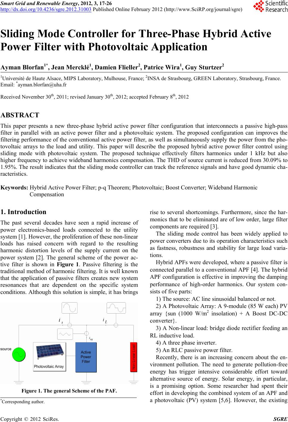
Smart Grid and Renewable Energy, 2012, 3, 17-26
http://dx.doi.org/10.4236/sgre.2012.31003 Published Online February 2012 (http://www.SciRP.org/journal/sgre)
17
Sliding Mode Controller for Three-Phase Hybrid Active
Power Filter with Photovoltaic Application
Ayman Blorfan1*, Jean Mercklé1, Damien Flieller2, Patrice Wira1, Guy Sturtzer2
1Université de Haute Alsace, MIPS Laboratory, Mulhouse, France; 2INSA de Strasbourg, GREEN Laboratory, Strasbourg, France.
Received November 30th, 2011; revised January 30th, 2012; accepted February 8th, 2012
ABSTRACT
This paper presents a new three-phase hybrid active power filter configuration that interconnects a passive high-pass
filter in parallel with an active power filter and a photovoltaic system. The proposed configuration can improves the
filtering performance of the conventional active power filter, as well as simultaneously supply the power from the pho-
tovoltaic arrays to the load and utility. This paper will describe the proposed hybrid active power filter control using
sliding mode with photovoltaic system. The proposed technique effectively filters harmonics under 1 kHz but also
higher frequency to achieve wideband harmonics compensation. The THD of source current is reduced from 30.09% to
1.95%. The result indicates that the sliding mode controller can track the reference signals and have good dynamic cha-
racteristics.
Keywords: Hybrid Active Power Filter; p-q Theorem; Photovoltaic; Boost Converter; Wideband Harmonic
Compensation
1. Introduction
The past several decades have seen a rapid increase of
power electronics-based loads connected to the utility
system [1]. However, the proliferation of these non-linear
loads has raised concern with regard to the resulting
harmonic distortion levels of the supply current on the
power system [2]. The general scheme of the power ac-
tive filter is shown in Figure 1. Passive filtering is the
traditional method of harmonic filtering. It is well known
that the application of passive filters creates new system
resonances that are dependent on the specific system
conditions. Although this solution is simple, it has brings
Figure 1. The general Scheme of the PAF.
rise to several shortcomings. Furthermore, since the har-
monics that to be eliminated are of low order, large filter
components are required [3].
The sliding mode control has been widely applied to
power converters due to its operation characteristics such
as fastness, robustness and stability for large load varia-
tions.
Hybrid APFs were developed, where a passive filter is
connected parallel to a conventional APF [4]. The hybrid
APF configuration is effective in improving the damping
performance of high-order harmonics. Our system con-
sists of five parts:
1) The source: AC line sinusoidal balanced or not.
2) A Photovoltaic Array: A 9-module (85 W each) PV
array {sun (1000 W/m2 insolation) + A Boost DC-DC
converter}.
3) A Non-linear load: bridge diode rectifier feeding an
RL inductive load.
4) A three phase inverter.
5) An RLC passive power filter.
Recently, there is an increasing concern about the en-
vironment pollution. The need to generate pollution-free
energy has trigger intensive considerable effort toward
alternative source of energy. Solar energy, in particular,
is a promising option. Some researcher had spent their
effort in developing the combined system of an APF and
a photovoltaic (PV) system [5,6]. However, the existing
*Corresponding author.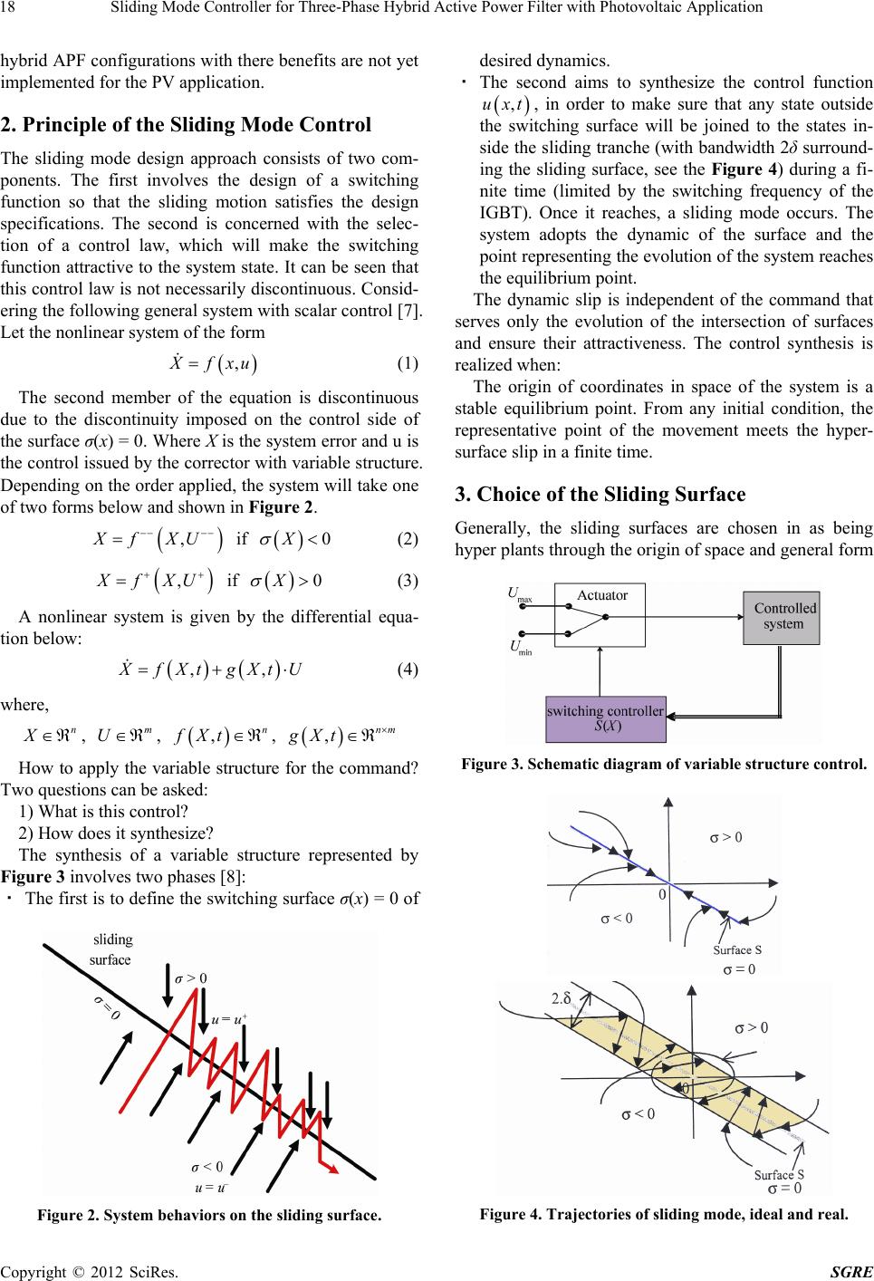

Sliding Mode Controller for Three-Phase Hybrid Active Power Filter with Photovoltaic Application
18
hybrid APF configurations with there benefits are not yet
implemented for the PV application.
2. Principle of the Sliding Mode Control
The sliding mode design approach consists of two com-
ponents. The first involves the design of a switching
function so that the sliding motion satisfies the design
specifications. The second is concerned with the selec-
tion of a control law, which will make the switching
function attractive to the system state. It can be seen that
this control law is not necessarily discontinuous. Consid-
ering the following general system with scalar control [7].
Let the nonlinear system of the form


,
X
fxu
 (1)
The second member of the equation is discontinuous
due to the discontinuity imposed on the control side of
the surface σ(x) = 0. Where X is the system error and u is
the control issued by the corrector with variable structure.
Depending on the order applied, the system will take one
of two forms below and shown in Figure 2.

,Xf XU
 
 if (2)

0X  

,
X
fXU

 if (3)

0X  
A nonlinear system is given by the differential equa-
tion below:

,,
X
fXt gXtU
 (4)
where,
n
X , , ,
m
U

,n fXt

,nm gXt


How to apply the variable structure for the command?
Two questions can be asked:
1) What is this control?
2) How does it synthesize?
The synthesis of a variable structure represented by
Figure 3 involves two phases [8]:
· The first is to define the switching surface σ(x) = 0 of
Figure 2. System behaviors on the sliding surface.
desired dynamics.
· The second aims to synthesize the control function


,uxt, in order to make sure that any state outside
the switching surface will be joined to the states in-
side the sliding tranche (with bandwidth 2δ surround-
ing the sliding surface, see the Figure 4) during a fi-
nite time (limited by the switching frequency of the
IGBT). Once it reaches, a sliding mode occurs. The
system adopts the dynamic of the surface and the
point representing the evolution of the system reaches
the equilibrium point.
The dynamic slip is independent of the command that
serves only the evolution of the intersection of surfaces
and ensure their attractiveness. The control synthesis is
realized when:
The origin of coordinates in space of the system is a
stable equilibrium point. From any initial condition, the
representative point of the movement meets the hyper-
surface slip in a finite time.
3. Choice of the Sliding Surface
Generally, the sliding surfaces are chosen in as being
hyper plants through the origin of space and general form
Figure 3. Schematic diagram of variable structure control.
Figure 4. Trajectories of sliding mode, ideal and real.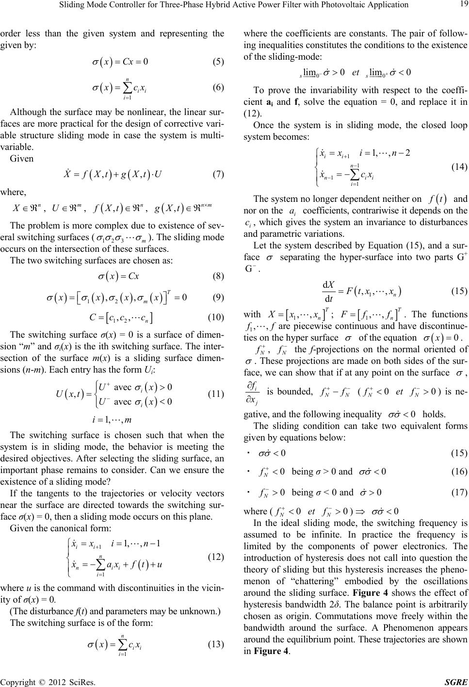

Sliding Mode Controller for Three-Phase Hybrid Active Power Filter with Photovoltaic Application 19
order less than the given system and representing the
given by:

0xCx 

 (5)

1
n
ii
i
x
cx 



(6)
Although the surface may be nonlinear, the linear sur-
faces are more practical for the design of corrective vari-
able structure sliding mode in case the system is multi-
variable.
Given




,,
X
fXt gXtU
 (7)
where,
n
X , , ,
m
U

,n fXt

,nm gXt


The problem is more complex due to existence of sev-
eral switching surfaces (123 m

  ). The sliding mode
occurs on the intersection of these surfaces.
The two switching surfaces are chosen as:

x
Cx   (8)
 
12
,, T
m
xxxx   

0 (9)


12
,, n Ccc c (10)
The switching surface σ(x) = 0 is a surface of dimen-
sion “m” and σi(x) is the ith switching surface. The inter-
section of the surface m(x) is a sliding surface dimen-
sions (n-m). Each entry has the form Ui:
 

avec 0
, avec 0
i
i
Ux
Uxt Ux








 (11)
1, ,im
The switching surface is chosen such that when the
system is in sliding mode, the behavior is meeting the
desired objectives. After selecting the sliding surface, an
important phase remains to consider. Can we ensure the
existence of a sliding mode?
If the tangents to the trajectories or velocity vectors
near the surface are directed towards the switching sur-
face σ(x) = 0, then a sliding mode occurs on this plane.
Given the canonical form:

1
1
1, ,1
ii
n
nii
i
xx in
x
axf tu





 





(12)
where u is the command with discontinuities in the vicin-
ity of σ(x) = 0.
(The disturbance f(t) and parameters may be unknown.)
The switching surface is of the form:

1
n
ii
i
x
cx 



(13)
where the coefficients are constants. The pair of follow-
ing inequalities constitutes the conditions to the existence
of the sliding-mode:
0
lim 0
s




 et 0
lim 0
s




To prove the invariability with respect to the coeffi-
cient ai and f, solve the equation = 0, and replace it in
(12).
Once the system is in sliding mode, the closed loop
system becomes:
1
1
1
1
1, ,2
ii
n
nii
i
xx in
xcx











 (14)
The system no longer dependent neither on


f
t and
nor on the i coefficients, contrariwise it depends on the
i, which gives the system an invariance to disturbances
and parametric variations.
a
c
Let the system described by Equation (15), and a sur-
face

separating the hyper-surface into two parts G+
G

.

1
d,, ,
dn
X

F
tx x
t (15)
with

1,, T n
X
xx;

1,, T n

F
ff. The functions
1are piecewise continuous and have discontinue-
ties on the hyper surface
,,ff

of the equation


0x 

.
N
f

,
N
f

the f-projections on the normal oriented of

. These projections are made on both sides of the sur-
face, we can show that if at any point on the surface

,
i
j
f
x


is bounded,
N
N
f
f


 ( et ) is ne- 0
N
f0
N
f
gative, and the following inequality 0

 
 holds.
The sliding condition can take two equivalent forms
given by equations below:
· 0



 (15)
· 0
N
f

being σ > 0 and 0

 
 (16)
· 0
N
f being σ < 0 and 0


 (17)
where (0
N
f

et )  0
N
f0

 

In the ideal sliding mode, the switching frequency is
assumed to be infinite. In practice the frequency is
limited by the components of power electronics. The
introduction of hysteresis does not call into question the
theory of sliding but this hysteresis increases the pheno-
menon of “chattering” embodied by the oscillations
around the sliding surface. Figure 4 shows the effect of
hysteresis bandwidth 2δ. The balance point is arbitrarily
chosen as origin. Commutations move freely within the
bandwidth around the surface. A Phenomenon appears
around the equilibrium point. These trajectories are shown
in Figure 4.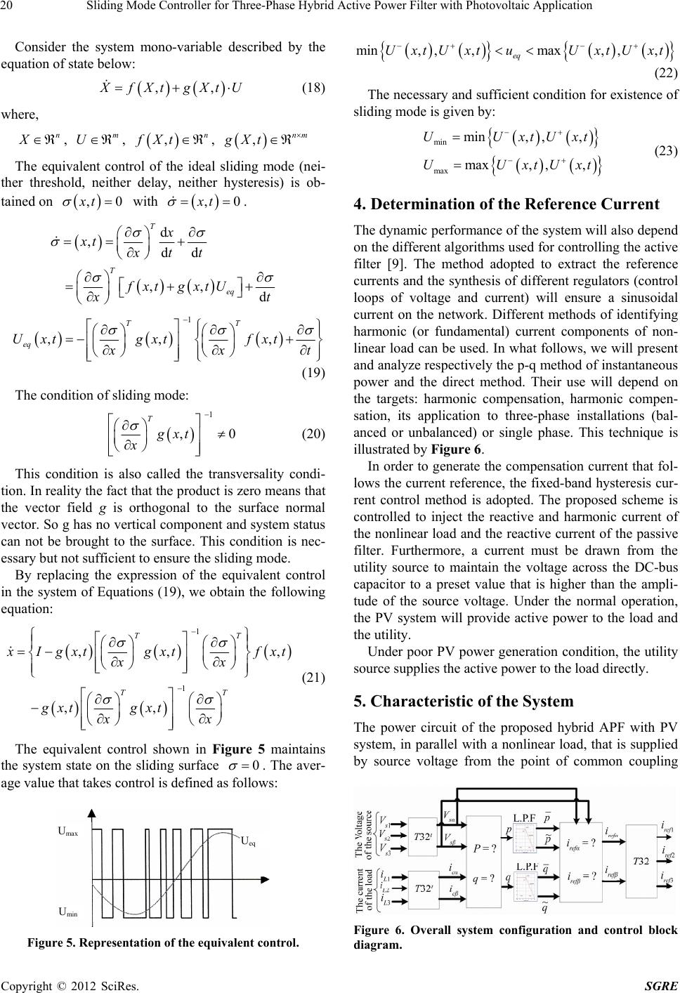

Sliding Mode Controller for Three-Phase Hybrid Active Power Filter with Photovoltaic Application
20
Consider the system mono-variable described by the
equation of state below:




,,
X
fXt gXtU

(18)
where,
n
X , , ,
m
U

,n fXt

,nm gXt


The equivalent control of the ideal sliding mode (nei-
ther threshold, neither delay, neither hysteresis) is ob-
tained on with .

,xt  0

,0xt  


 
d
,dd
,,d
T
T
eq
x
xt xtt
fxt gxtU
x
t






 














  
1
,,,
TT
eq
Uxt gxt fxt
x
xt




 
 
 


 

 
 



 




(19)
The condition of sliding mode:

1
,
T
gxt
x




 






0 (20)
This condition is also called the transversality condi-
tion. In reality the fact that the product is zero means that
the vector field g is orthogonal to the surface normal
vector. So g has no vertical component and system status
can not be brought to the surface. This condition is nec-
essary but not sufficient to ensure the sliding mode.
By replacing the expression of the equivalent control
in the system of Equations (19), we obtain the following
equation:
 
 
1
1
,,
,,
TT
TT
,
x
Igxt gxtfxt
xx
gxt gxt
xx








 
 

 

 

















(21)
The equivalent control shown in Figure 5 maintains
the system state on the sliding surface 0

. The aver-
age value that takes control is defined as follows:
Figure 5. Representation of the equivalent control.










min, ,,max, ,,
eq
UxtUxtuUxtUxt
 

(22)
The necessary and sufficient condition for existence of
sliding mode is given by:
 


 

min
max
min, ,,
max, ,,
UUxtUx
UUxtU




t
xt
(23)
4. Determination of the Reference Current
The dynamic performance of the system will also depend
on the different algorithms used for controlling the active
filter [9]. The method adopted to extract the reference
currents and the synthesis of different regulators (control
loops of voltage and current) will ensure a sinusoidal
current on the network. Different methods of identifying
harmonic (or fundamental) current components of non-
linear load can be used. In what follows, we will present
and analyze respectively the p-q method of instantaneous
power and the direct method. Their use will depend on
the targets: harmonic compensation, harmonic compen-
sation, its application to three-phase installations (bal-
anced or unbalanced) or single phase. This technique is
illustrated by Figure 6.
In order to generate the compensation current that fol-
lows the current reference, the fixed-band hysteresis cur-
rent control method is adopted. The proposed scheme is
controlled to inject the reactive and harmonic current of
the nonlinear load and the reactive current of the passive
filter. Furthermore, a current must be drawn from the
utility source to maintain the voltage across the DC-bus
capacitor to a preset value that is higher than the ampli-
tude of the source voltage. Under the normal operation,
the PV system will provide active power to the load and
the utility.
Under poor PV power generation condition, the utility
source supplies the active power to the load directly.
5. Characteristic of the System
The power circuit of the proposed hybrid APF with PV
system, in parallel with a nonlinear load, that is supplied
by source voltage from the point of common coupling
Umax Ueq
Umin
Figure 6. Overall system configuration and control block
diagram.

Sliding Mode Controller for Three-Phase Hybrid Active Power Filter with Photovoltaic Application
21
PCC. The proposed hybrid APF consists of a passive
high-pass filter (HPF), a shunt APF constructed by a
three-phase full-bridge voltage source inverter (VSI)
connected to a DC-bus capacitor; and PV arrays in par-
allel with the DC-bus capacitor. In the proposed scheme,
the low order harmonics are compensated using the shunt
APF, while the high-order harmonics are filtered with the
passive HPF. This configuration is effective to improve
the filtering performance of the high-order harmonics.
The inverter is shown in Figure 7.
10 A
n
d
d
S
IV  , 52
d
d
d
V
RI 
The inductor L has a value between 1% and 10% of
the nominal value of inductance L is defined by:
1
s
c
V
L
I

 with 1
2
3
cd
I
I
The term 1c
I
represents the effective value of the
fundamental component of the load current c
I
and

the pulse of the electrical network.
The simplest solar cell model consists of diode and
current source parallel connected. Source current is di-
rectly proportional to the solar radiation. Diode repre-
sents PN junction of a solar cell.
6. Control the Switching Frequency
P
VSC
iIi
D
(24)
00
1
D
T
V
eV
V
KT 1
L
D
iIeI iIeI

 


 
 
(25)
The parametric study has confirmed that the switching
frequency is strongly dependent on coupling inductance
Lf and width of hysteresis band. The objective of this
part is to propose a method to limit the frequency swi-
tching and make it independent of parametric variations.
For this, we propose to add to the expression of the surface
a triangular signal whose frequency is constant and the
amplitude is fixed. The principle of the method is il-
lustrated in Figure 10.
The proposed model of a photovoltaic cell using Mat-
lab is shown by Figure 8.
The photovoltaic system consists of:
1) A 9-module (85 W each) PV array with full sun
(1000 W/m2 insolation); 7. Simulation Results
2) A Boost DC-DC converter that steps-up a DC input
voltage; The proposed hybrid APF was simulated using MAT-
3) A capacitor C under DC voltage that provides nec-
essary energy storage to balance instantaneous power de-
livered to the grid.
The photovoltaic system is shown by Figure 9.
The pollution load is materialized by a bridge diode
rectifier feeding an RL inductive load. The network is
modeled by three perfect sinusoidal voltage sources in
series with an inductance Ls and resistance Rs Bridge
operates under a simple rms voltage of 220 V and con-
sumes a power rating of 5.2 KVA. We deduce the fol-
lowing characteristic quantities for the nonlinear load:
36
514.86 V
π
s
d
V
V  , Figure 7. Structure of the inverter.
Figure 8. Model of PV cell using simulink.

Sliding Mode Controller for Three-Phase Hybrid Active Power Filter with Photovoltaic Application
22
Figure 9. Model of PV using simulink.
Figure 10. Principle of limiting the switching frequency.
LAB Simulink program. The system parameters are shown
in following table. In the simulation, a diode rectifier
with a DC-link capacitor and a smoothing inductor was
used as a harmonic producing nonlinear load.
The proposed scheme is shown in Figure 11. Now, the
high-order harmonics are filtered from the source voltage
and source current. The sufficient condition for existence
of sliding regimes is the following:
2
3
2
3
d
q
u
u









(26)
This condition depends on the values chosen for the
DC bus voltage VC and the coupling inductance of the
inverter network (Lf).
The conditions of Equation (26) give:

32
23
cos
32
23
c
c
Lf Id
VVm
Id
VLf




















(27)
The equivalent control is then given by:
Matlab Simulink Simulation Parameters
Utility Voltage 2202 (50 Hz)
Source Inductance 0.65e–3 H
Source Resistance 5–3 Ω
Rectifier Smoothing Inductor 1–3 H
Rectifier Smoothing Resistance 1.5 Ω
Load Inductance 100–3 H
Load Resistance 29 × 1.5 Ω
Load Capacitance 2000–6 F
Current Control Band 1.8 A
Sampling Time 10–6 s
APF Inductor 2–3 H
APF Resistor 0.005 Ω
APF DC-Bus Capacitor 450 V
HPF Capacitor 5.01e–6 F
HPF Resistor 20.46 Ω
PV 9 arrays
INSOLATION 1000 w/m2
Short-Circuit Current Isc 5.45 A
Open-Circuit Voltage Voc 22.2 V
Rated Current IR at Maximum Power Point (MPP)4.95 A
Rated Voltage VR at MPP 17.2 V
Capacitance of the PV Output 2–3 F
Resistance of PV Output 72.78 Ω
d
dd
d
dd
ffd f
Sd
deqfd fq
cf
ffd f
Sd
qeqfd fq
cf
LI R
V
uI
VttL
LI R
V
uI
VttL












I
I
(28)

Sliding Mode Controller for Three-Phase Hybrid Active Power Filter with Photovoltaic Application 23
Figure 11. Complete diagram of the control structure
In order to ensure the sliding mode, the value of Vc
must take the maximum of these two values.
We put:
3
arcsin 2qeq u 





and 3 arccos 2deq u 



The source currents after compensation are almost sin-
usoidal and in phase with the voltage at the connection
point. The spectra of source current before and after
compensation are presented in Figures 12 and 14. The
total harmonic distortion (THD) current source (calcu-
lated on the first 30 harmonic orders) increased from
30.09% to 1.95% and the load current harmonic compo-
nents are greatly reduced. Note also that the DC bus
voltage is regulated to 700 V.
All results are shown in Figure 13 (The source, the
current of load before and after the compensation, in ad-
dition to the current of the filter and the DC voltage of
the capacitor).
Figure 14 shows the spectrum of the source current is
in dB. This spectrum allows us to see that the switching
frequency varies between 5 and 10 kHz. The average
switching frequency is equal to 9.07 kHz. Low frequency
peaks are located between –40 dB and –60 dB. Above 4
kHz, the amplitudes of the lines are growing and both the
frequency 7.5 kHz is reached, they are decreasing. Be-
yond 16 kHz, the spectrum is more regular and rays have
elative amplitudes below –50 dB. This spectrum is shown r

Sliding Mode Controller for Three-Phase Hybrid Active Power Filter with Photovoltaic Application
24
Frequency f (Hz)
Harmonic spectrum
Figure 12. Harmonic spectrum of source current before the compensation.
Vc(V)
Figure 13. Compensation of harmonic currents with the sliding mode control.
in Figure 15.
8. Conclusions
In order to improving of the current reference a signal
type sign was added to the equivalent control, the THD is
improved (reduced), but the average switching frequency
is slightly increased. To reduce the switching frequency
ithout changing system settings, a technique based on w

Sliding Mode Controller for Three-Phase Hybrid Active Power Filter with Photovoltaic Application 25
Harmonic spectrum
Frequency f (Hz)
Figure 14. Harmonic spectrum of source current after the compensation.
Frequency f (Hz)
Relative amplitude in dB
Figure 15. Spectrum of the source current is in dB.
the addition of a triangular signal to the switching surface
has been proposed and tested.
The simulation results show the effectiveness of the
proposed scheme for wideband harmonics compensation
and PV power handling capability. Combined with the
fastness and robustness of sliding mode control, HAPF
based on sliding mode control has good robustness and
stability. The loop for the capacitor voltage regulation is

Sliding Mode Controller for Three-Phase Hybrid Active Power Filter with Photovoltaic Application
26
introduced into the sliding mode control; good regulation
effect in DC bus is obtained for load variation.
REFERENCES
[1] H. Akagi, “Control Strategy of Active Power Filters Using
Multiple Voltage-Source PWM Converters,” IEEE Trans-
actions on Industry and Application, Vol. IA-22, No. 3,
1986, pp. 460-465.
[2] A. D. Ould, et al., “A Unified Artificial Neural Network
Architecture for Active Power Filters,” Industrial Electron-
ics IEEE Transactions on Industrial and Electronics, Vol.
54, No. 1, 2007, pp. 61-76. doi:10.1109/TIE.2006.888758
[3] A. H. S. Rahmani, N. Mendalek and K. Al-Haddad, “A
New Control Technique for Three-Phase Shunt Hybrid
Power Filter,” IEEE Transactions on Industrial Electronics,
Vol. 56, No. 8, 2009, pp. 2904-2915.
doi:10.1109/TIE.2008.2010829
[4] A. Hamadi, et al., “Sliding Mode Control of Three-Phase
Shunt Hybrid Power Filter for Current Harmonics Com-
pensation,” International Symposium on Industrial Elec-
tronics IEEE, Bari, 4-7 July 2010, pp. 1076-1082.
[5] A. Blorfan, D. Flieller, P. Wira, G. Sturtzer and J. Merckle,
“A New Approach for Modeling the Photovoltaic Cell
Using Orcad Comparing with the Model Done in Mat-
lab,” International Review on Modeling and Simulations,
Vol. 3, No. 5, 2010, pp. 948-954.
[6] X.-J. Dai and Q. Chao, “The Research of Photovoltaic
Grid-Connected Inverter Based on Adaptive Current
Hysteresis Band Control Scheme,” Proceedings of the
SUPERGEN International Conference on Sustainable
Power Generation and Supply, Shanghai, 6-7 April 2009,
pp. 1-8.
[7] P. Wang, B.-H. Cheng and Z.-B. Zhang, “Sliding Mode
Control for a Shunt Active Power Filter,” Proceedings of
the 3rd International Conference on Measuring Technol-
ogy and Mechatronics Automation, Shanghai, 6-7 January
2011, pp. 282-285. doi:10.1109/ICMTMA.2011.641
[8] B. Cheng, et al., “Sliding Mode Control for a Shunt Ac-
tive Power Filter,” Proceedings of the 3rd International
Conference on Measuring Technology and Mechatronics
Automation, Shanghai, 6-7 January 2011, pp. 282-285.
[9] B. R. Lin and T. Y. Yang, “Three-Level Voltage-Source
Inverter for Shunt Active Filter,” IEE Transactions on
Electric Power Applications, Vol. 151, No. 6, 2004, pp.
744-751.
Nomenclature
HAPF: Hybrid Active Power Filter
APF: Active Power Filter
PV: Photovoltaic
σ(x): Surface of Sliding
X: System Error
u: Control Variable
U: Control Vector
2δ: Bandwidth around the Sliding Surface
f, g: Functions of the Non Linear System
C: Coefficients of σ(x)