Journal of Mathematical Finance, 2012, 2, 31-37
http://dx.doi.org/10.4236/jmf.2012.21003 Published Online February 2012 (http://www.SciRP.org/journal/jmf)
On the Consistency of a Firm’s Value with a Lognormal
Diffusion Process
Andrew M. K. Cheung1, Van Son Lai2
1Department of Finance, Fairleigh Dickinson University, Vancouver, Canada
2Department of Finance, Laval University, Quebec City, Canada
Received November 12, 2011; revised December 10, 2011; accepted December 30, 2011
ABSTRACT
A partial equilibrium model is developed to examine conditions supporting the representation of the value of a firm by
the lognormal diffusion process. The model formalizes the operating side of the firm and leads to a formula valuing the
firm’s risky profit stream. The present value formula is then compared to the existing work on valuing exogenous risky
income stream. Implications of the resulted pricing model on the volatility of the firm value processes are explored.
Keywords: Cashflow Valuation; Adjustment Cost; Non-Constant Volatility Process; Lognormal Distribution
1. Introduction
Since the work of Merton [1] on pricing risky debt of a
firm, it becomes a standard in the finance literature to as-
sume a geometric Brownian motion representation of a
firm’s value process. Such a constant volatility lognormal
distribution, the horsepower of option pricing, is rather
consistent with some earlier influential papers by Rubin-
stein [2] and Ross [3]. These papers take the firm’s risky
investment cashflows as an exogenous stochastic process
and then value these future income streams via an in-
tertemporal arbitrary pricing operator.
In this paper, we explicitly model a firm that performs
intertemporal profit maximization. Our model assumes there
is a futures market for the firm’s output. It specifies an
internal production function for the firm and the adjust-
ment cost function for its investment. This specification
in conjunction with the external arbitrage market force leads
to a present value formula for the firm’s operating profit.
Compared to one of the key results of Rubinstein [2], our
main result unveils some severe restrictions behind the
exogenous cashflow approach to a firm’s value. Since the
literature on the term structure of defaultable debt based
on the constant volatility firm value process has not been
empirically supported (see for instance Schonbucher [4]),
our pricing formula also allows us to critically re-examine
the firm value process. The main feature of our model
imbeds a non-constant volatility value process while main-
taining the tractable spirit of the classic structural approach
to contingent claims analysis (CCA).
The rest of the paper is organized as follows. Section 2
describes the market setting. The firm’s production acti-
vity is introduced in Section 3. The present value of the
firm’s intertemporal profit and the resulting valuation
equations are developed in Section 4 to 5. Section 6 con-
cludes the paper.
2. The Market Setting
The analysis begins with a firm producing an output traded
in a perfectly competitive market. The output price is as-
sumed to follow an exogenous stochastic process
d = ddPPt z

  (1)
where dz is the increment to a standard Brownian motion
process,

represents the expected growth rate of the out-
put price and

stands for the instantaneous volatility of
the output price. Both

and

are assumed to be
constant values rendering the conditional output price to
be a lognormally distributed process.
Let F(P, t) denote the futures price at time t for deliv-
ery of one unit of the output at time T and use Tt



to represent the remaining time to maturity. By Ito’s le-
mma, the instantaneous change in the futures price is
given by


22
d=12d d.
PP P
F
FFPtF

  P (2)
The above equation represents the gains or losses gen-
erated by holding a futures contract. Uncertainty enters
into a futures position through the second term. The risky
component can be eliminated via a creation of the ac-
companying hedge portfolio. At time t an investor can
buy one unit of the commodity at a cost of P(t) and si-
multaneously take a short position of 1
P
F
 shares of
C
opyright © 2012 SciRes. JMF

A. M. K. CHEUNG ET AL. 32
futures contract. The futures position does not entail any
initial cost.
The value of the hedge portfolio in the next instant is
given by where the middle term
rewards the owner of the commodity with the conven-
ience of having the output on hand. In percentage terms,
the return to the hedge portfolio is given by
1
dd
P
PPtF F 

 d
 


122
dd d
d12
P
PPP
PPt PFF
tPFFF Pt





 d 
(3)
By virtue of the standard arbitrage argument forces the
above deterministic portfolio return to be identical to the
instantaneous return on the riskless asset drt

. This
implies the valuation partial differential equation (here-
after denoted as PDE) of the futures price is given by


122
d12d
PPP
tPFFFPt rt



 d.
Upon simplifying, we have

22
12 0.
P PP
FPr PFF

   (4)
It can be readily verified that the solution to the PDE
takes a simple form:
 
,expFPtPtr.

  
 
(5)
The following relation, a stochastic representation of
the futures price process, is useful for the subsequent
development of our main result:


dd
PP
d
F
FPPFrt  . (6)
3. The Firm’s Operating Profit
The firm is assumed to operate in a perfectly competitive
output market where there is no tax and the output fluc-
tuates according to the geometric Brownian motion
process. The firm’s instantaneous revenue at time s is
generated by P(s)Q(s) where Q(s) is the firm’s produc-
tion function taking labor and capital as the input factors.
We assume the firm’s labor choice L(s) can be made in-
stantaneously whereas the adjustment cost assumption
prohibits the firm to immediately obtain the desired
capital stock.
Denote the investment variable as I(t) and the capital
stock K(t); the relationship between these is defined by
dK = I(t)dt. The cost function associated with a given
level of I(t) is defined by C(I). We assume that C(I) is a
convex cost function which is increasing in investment,
such that and

0CI



0.CI
  Convexity of the
cost function captures the reality that a high level of in-
vestment extracts limited resources from the firm to pre-
pare for installation of additional capital stocks or to train
labors with newly acquired machines. A convex adjust-
ment cost function plays a key role in determining a fi-
nite size of the firm. Physical depreciation rate can be
incorporated to the above stock and flow relation. How-
ever, for simplicity of exposition, we assume no depre-
ciation.
Given the output of the firm at each instant, Q(K,L), its
net profit at time t is defined by the difference between
sales revenue and the relevant costs involved in produc-
ing the output:






π,tPtQKLwLtCI


(7)
While the management chooses the current level of
labor combined with existing capital stocks to generate
highest possible revenue, it has to devote resources to
prepare for the future level of capital stocks in its pro-
duction activity. The last term in the net profit equation
for the firm then creates an intertemporal link between the
current profit and the future profit for the firm, given the
entire lifespan of the company, via the differential equa-
tion for the stock variable K(t). Given the instantaneously
adjustable choice variable L and dynamic control vari-
able I, the management takes the stochastic output price
process P(t) as the exogenous state variable. In this com-
plete futures market, risk preference does not play a role
in valuing the intertemporal profit of the business.
This implies there exists an equivalent martingale mea-
sure so that the firm evaluates its risky profit stream by
using the risk free rate to discount the conditional expec-
tation of its future net cash flow with respect to this mar-
tingale measure.
Maximization of the firm’s net present value can be
expressed as




  

,
,
max exp,d
T
I
L t
t
VKt t
ErtPsQLKwLCIs


 

(8)
where t

represents the information set generated by
the commodity price P(t) and the expectation is taken
with respect to the equivalent martingale measure. When
the price process is specified as a lognormal diffusion,
the information set can be substantially simplified. In this
case t

can be replaced by the currently observed
value of the price process, P(t).
4. The Arbitrage Valuation of the Firm’s
Income Stream
The net present value function indicates the business
profit is derived from producing the homogeneous product
that is sold at the market determined price P. At any
future instant, the firm’s profit is defined by combining
the output price process with its production function. The
valuation of these uncertain profit stream is parallel to
that of determining the futures price in the earlier section.
Denote the present value of the firm by G(P,K,t). Con-
sider the return to a hedge portfolio consisting of owning

A. M. K. CHEUNG ET AL. 33
one unit of the firm’s share and a short position on
P
P
GF futures contracts. As the value of the firm is
governed by the three state variables K and P and t,
application of Ito’s lemma leads to
maximizing activities. Unless the production is under
decreasing return to scale, the size of the firm in this case
will end up being indeterminate. The other extreme,


, captures the firm’s capacity constraint; any
capital expansion is met with an infinite expense incurred
by the firm’s operation.

2
dddd12d
PK tPP
GGPGKGtG P , (9)
Letting

fall between the two extreme parametric
values, the constant parameter

can be interpreted as
a measure of the speed of adjustment to the newly
installed capital stocks. The case of a linear cost function
where 1


, when combined with a constant return to
scale production function leads to a firm’s profit function
that is linear in the capital stock. The implication of having
a linear adjustment cost function is that the speedy capital
formation indicates an unbounded acquisition of new
capital to maximize the firm’s profit. The resulting firm’s
size is again indeterminate. The convex adjustment cost,
represented by 1

, can be justified as placing a bound
to the firm’s size. The chosen adjustment cost function is
then combined with the firm’s production technology.
where the last term captures the Jensen’s inequality
representing the plausible non-linear relation between the
firm’s value and the output price. Recalling that the firm’s
current profit from producing the output is given by
we add these terms as income con-
tributions to obtain the total change in the firm’s value.
On the other hand, the short futures position in the hedge
portfolio generates the payoff given by

,PQwL CI

d.
PP
GF F
Combining the instantaneous value changes in each
component of the hedge portfolio leads to
 


2
2
dd12d
dd
dd12d
d.
PK PP
PP
Kt PP
GPGItGP
PQwLCItGFF
GIt GtGPtrPGt
PQwLC It


  

 
 

d
P
The latter is assumed to be the Cobb-Douglas pro-
duction function
 
1
,,QKLLtKt

 
 where

is assumed to be a constant and 01

.
The right side of the above equation results from sub-
stituting the expressions for dP and dF from Equations (1)
and (8) and simplifying. This equality indicates that the
hedged portfolio return is non-stochastic. In the absence
of arbitrage opportunity, the hedge portfolio return must
grow at the riskfree rate leading to the following valu-
ation PDE:
The above specification of the investment cost function
and the production technology reduce the generality of
our model but it is motivated by the search for a closed
form solution to the valuation problem. To further
enhance the tractability of the problem, we assume that
the firm is infinitely long-lived, removing the calendar
time as one of the three state variables in the partial
differential equation. The consequent valuation PDE
derived from the last section is reduced to


22
12 PPP K
t
PGrGG I
GPQwLCI rG
  
  (10)




22
1
,
12
max.
PP P
IL K
rGPGrP G
GIPLKwLI
 





(11)
The solution function G(P,K,t) to the partial differential
equation represents the present value of the firm under a
defined operating policy. The space of solution functions
can be narrowed down and the solution form can be
sharpened as soon as optimal choices to the control are
made in the firm’s decision problem and appropriate
boundary conditions are specified.
Performing the required maximization and substituting
the resulting optimal choices yield the nonlinear PDE


 
 
22
11 11
12
1
PP P
K
rGPGrPG
GP







 


K
(12)
5. The Solution to the Profit Maximization
Problem and the Value of the Firm
where



11
1w



 .
The above valuation
equation for the firm’s value is expressed in terms of the
state variables P and K given the parameters of the
production and cost functions. Appendix A shows that
the above valuation PDE has a solution given by
This paper assumes a parametric form for the adjustment
cost function
 
, 0 and 1.CI It

  


0,  
The parameter measures the significance
of the adjustment cost. When 0

, adjustment cost
does not play any role in determining the firm’s profit
  



  

1
2
2
1
,
112111
GKPK
r


 



 
2
(13)

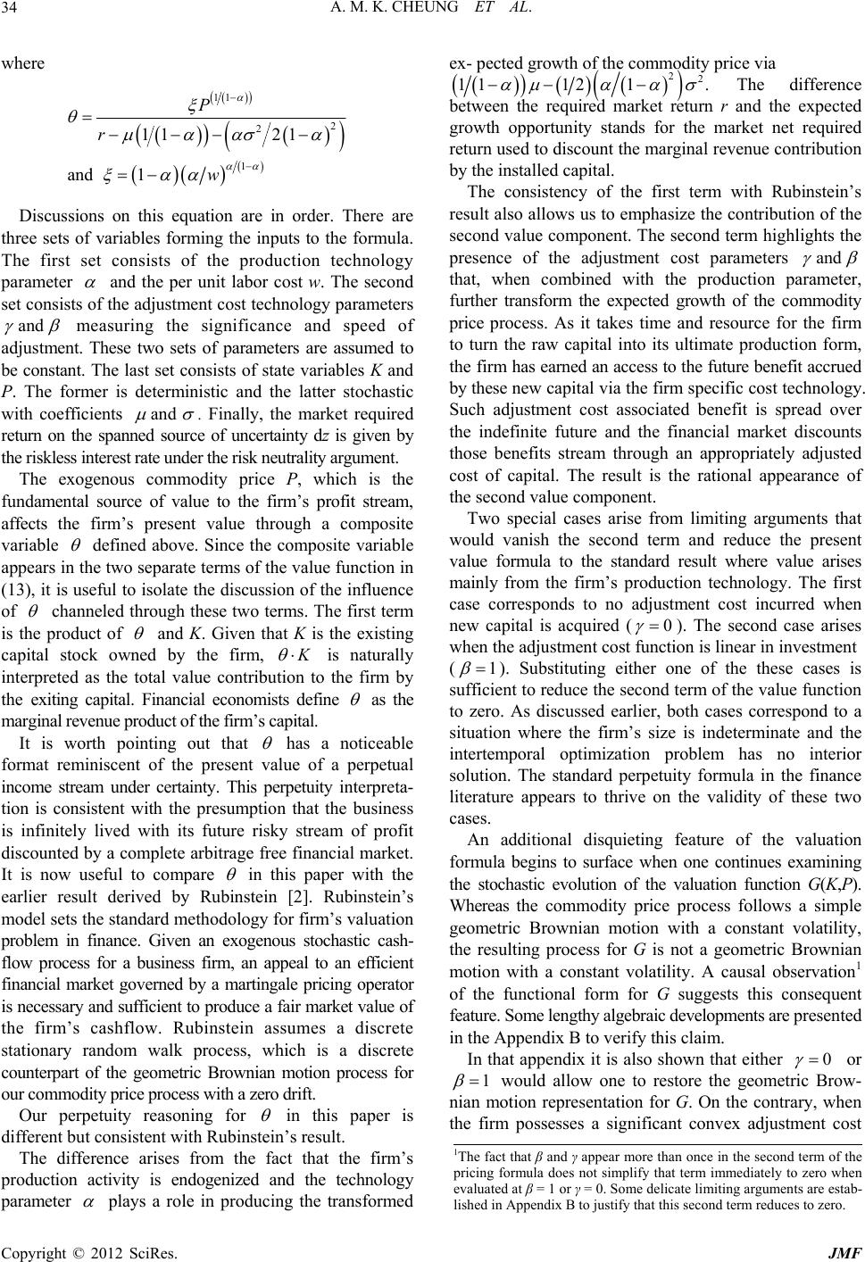
A. M. K. CHEUNG ET AL. 34
where
 
  



11
2
2
1
11 21
and 1
P
r
w



 





Discussions on this equation are in order. There are
three sets of variables forming the inputs to the formula.
The first set consists of the production technology
parameter

and the per unit labor cost w. The second
set consists of the adjustment cost technology parameters
and

measuring the significance and speed of
adjustment. These two sets of parameters are assumed to
be constant. The last set consists of state variables K and
P. The former is deterministic and the latter stochastic
with coefficients and

 . Finally, the market required
return on the spanned source of uncertainty dz is given by
the riskless interest rate under the risk neutrality argument.
The exogenous commodity price P, which is the
fundamental source of value to the firm’s profit stream,
affects the firm’s present value through a composite
variable

defined above. Since the composite variable
appears in the two separate terms of the value function in
(13), it is useful to isolate the discussion of the influence
of

channeled through these two terms. The first term
is the product of

and K. Given that K is the existing
capital stock owned by the firm,
K

 is naturally
interpreted as the total value contribution to the firm by
the exiting capital. Financial economists define

as the
marginal revenue product of the firm’s capital.
It is worth pointing out that

has a noticeable
format reminiscent of the present value of a perpetual
income stream under certainty. This perpetuity interpreta-
tion is consistent with the presumption that the business
is infinitely lived with its future risky stream of profit
discounted by a complete arbitrage free financial market.
It is now useful to compare

in this paper with the
earlier result derived by Rubinstein [2]. Rubinstein’s
model sets the standard methodology for firm’s valuation
problem in finance. Given an exogenous stochastic cash-
flow process for a business firm, an appeal to an efficient
financial market governed by a martingale pricing operator
is necessary and sufficient to produce a fair market value of
the firm’s cashflow. Rubinstein assumes a discrete
stationary random walk process, which is a discrete
counterpart of the geometric Brownian motion process for
our commodity price process with a zero drift.
Our perpetuity reasoning for

in this paper is
different but consistent with Rubinstein’s result.
The difference arises from the fact that the firm’s
production activity is endogenized and the technology
parameter

plays a role in producing the transformed
ex- pected growth of the commodity price via
   


22
1112 1.

   
The difference
between the required market return r and the expected
growth opportunity stands for the market net required
return used to discount the marginal revenue contribution
by the installed capital.
The consistency of the first term with Rubinstein’s
result also allows us to emphasize the contribution of the
second value component. The second term highlights the
presence of the adjustment cost parameters and

that, when combined with the production parameter,
further transform the expected growth of the commodity
price process. As it takes time and resource for the firm
to turn the raw capital into its ultimate production form,
the firm has earned an access to the future benefit accrued
by these new capital via the firm specific cost technology.
Such adjustment cost associated benefit is spread over
the indefinite future and the financial market discounts
those benefits stream through an appropriately adjusted
cost of capital. The result is the rational appearance of
the second value component.
Two special cases arise from limiting arguments that
would vanish the second term and reduce the present
value formula to the standard result where value arises
mainly from the firm’s production technology. The first
case corresponds to no adjustment cost incurred when
new capital is acquired (0


). The second case arises
when the adjustment cost function is linear in investment
(1


). Substituting either one of the these cases is
sufficient to reduce the second term of the value function
to zero. As discussed earlier, both cases correspond to a
situation where the firm’s size is indeterminate and the
intertemporal optimization problem has no interior
solution. The standard perpetuity formula in the finance
literature appears to thrive on the validity of these two
cases.
An additional disquieting feature of the valuation
formula begins to surface when one continues examining
the stochastic evolution of the valuation function G(K,P).
Whereas the commodity price process follows a simple
geometric Brownian motion with a constant volatility,
the resulting process for G is not a geometric Brownian
motion with a constant volatility. A causal observation1
of the functional form for G suggests this consequent
feature. Some lengthy algebraic developments are presented
in the Appendix B to verify this claim.
In that appendix it is also shown that either 0


or
1


would allow one to restore the geometric Brow-
nian motion representation for G. On the contrary, when
the firm possesses a significant convex adjustment cost
1The fact that β and γ appear more than once in the second term of the
p
ricing formula does not simplify that term immediately to zero when
evaluated at β = 1 or γ = 0. Some delicate limiting arguments are estab-
lished in Appendix B to justify that this second term reduces to zero.

A. M. K. CHEUNG ET AL. 35
function, one does not have a lognormal diffusion
representation for its value process. The implication of
this analysis has some nontrivial bearing on many existing
models that rely on assuming a value process for a firm’s
assets following a geometric Brownian motion with a
constant volatility. Although the popular lognormal
diffusion model gives rise to numerous useful mathematical
features and valuable economic insights in finance, our
analysis has uncovered the severe limitations imposed on
the business entity when the constant volatility assumption
is adopted.
6. Conclusions
This paper begins with a neoclassic firm model and
explores conditions leading to the lognormal diffusion
price process that becomes the standard exogenous
stochastic process in modeling a firm’s value process
since the work of Merton [1]. There are works in finance
literature that traces the economic connection between
the lognormal diffusion process and the general equilibrium
fundamentals. Such interesting connection is essentially
behind the term viable price process after Bick’s [5]
influential analysis. The result of this paper is based on a
partial equilibrium firm value model in a complete market
setup which keeps the representative agent behind the risk
neutral probability. In the end, the geometric Brownian
motion value process with a constant volatility emerges
as a special case of a more general adjustment cost
technology. The resulting non-geometric Brownian motion
value process can also be qualified as a viable firm value
process.
In standard option pricing models, the assumption that
stock prices follow a geometric Brownian motion processes
has long been criticized as lacking empirical supports.
Proponents of the non-constant volatility model emphasize
the need to add random volatility and jumps in the
generalization of the original Black-Scholes model. The
notion that volatility is a non-diversifiable exogenous
process turns the original Black-Scholes option pricing
environment into an extended two state variables pricing
framework.
Earlier works of Hull and White [6], Scott [7] and
Heston [8], while offering substantial insights to the
extended pricing framework, add necessary economic
and computational complications. This paper is aligned
with the extended constant volatility literature, but it
aims at producing a tractable result on a firm’s value
with only one state variable. The next task is to take the
implication of the present paper to modify some of the
existing works that are crucially based on a geometric
Brownian motion process for the firm asset values, the
horsepower of Merton [1] seminal structural approach to
corporate securities.
7. Acknowledgements
The comments from Matthew Morin on an earlier draft
of this paper and the formatting assistance from Arsia As-
sadipour are greatly appreciated. Lai acknowledges financial
support from the Fonds Conrad Leblanc and the Social Sci-
ences and Humanities Research Council of Canada (SSH
RC).
REFERENCES
[1] R. C. Merton, “On the Pricing of Corporate Debt: The
Risk Structure of Interest Rates,” Journal of Finance, Vol.
29, No. 2, 1974, pp. 449-470. doi:10.2307/2978814
[2] M. Rubinstein, “The Valuation of Uncertain Income Streams
and the Pricing of Options,” Bell Journal of Economics
and Management Science, Vol. 7, 1976, pp. 407-425.
[3] S. A. Ross, “A Simple Approach to the Valuation of Ris-
ky Streams,” Journal of Business, Vol. 51, No. 3, 1978, pp.
453-475. doi:10.1086/296008
[4] P. J. Schonbucher, “Credit Derivatives Pricing Models,”
John Wiley and Sons, New York, 2003.
[5] A. Bick, “On the Consistency of Black Scholes Model with
a General Equilibrium Framework,” Journal of Financial
and Quantitative Analysis, Vol. 22, No. 3, 1987, pp. 259-
275. doi:10.2307/2330962
[6] J. C. Hull and A. White, “The Pricing of Options on Assets
with Stochastic Volatilities,” Journal of Finance, Vol. 42,
No. 2, 1987, pp. 218-300. doi:10.2307/2328253
[7] L. O. Scott, “Option Prices When the Variance Changes
Randomly,” Journal of Financial and Quantitative Analy-
sis, Vol. 22, No. 4, 1987, pp. 419-438.
doi:10.2307/2330793
[8] S. Heston, “A Closed Form Solution for Options with
Stochastic Volatility with Applications to Bond and Cu-
rrency Options,” Review of Financial Studies, Vol. 6, No.
2, 1993, pp. 327-345. doi:10.1093/rfs/6.2.327
[9] R. Goldberg, “Methods of Real Analysis,” John Wiley
and Sons, New York, 1976.

A. M. K. CHEUNG ET AL. 36
Appendix A
In this appendix we derive the solution to the non-linear
PDE stated as Equation (12) in Section 5. We conjecture
the following solution function
 
,GKPAPKBP
where A(P) and B(P) are functions assumed to be at least
twice continuously differentiable with respect to the va-
riable P. Then the valuation PDE take an additively
separable form
 



  


22
11 22
11
12
12
11
PP
PP
rAPKBPA KP
AK rPPKBP
Br PA
P

.
P



 
 



 







First adopt a functional form


11
AP qP



 and
we need to verify it satisfies the first segment of the en-
tire PDE. It is a matter of taking the necessary partial
derivatives, substituting the A(P) and its derivatives on
both sides of the above PDE. Then the unknown co-effi-
cient q comes out to be
    
22
1.
11 1211
q
rr



Finally, substitute q back into the conjectured solution
gives


 
 


11
22
1
11 1211
AP
P
rr


 

 
We have half of the solution for G(P,K) worked out as




,GPKAPKBPK BP  

where

is the chosen notation in Section 5 and it is
identical to A(P). It remains to solve for B(P). Let us
conjecture B(P) with the following solution form
 





1
11
11
11 BP bqP
bHP



 





where we set



1
11Hq

 



Next, substitute B(P) into the remaining segment of
the PDE with the corresponding partial derivatives appro-
priately taken in order to solve for the unknown coeffi-
cient b. The resulted b comes out to be
  

22
2
1
11121 1
b
rr

 
1
Further, putting b back into the conjectured solution B(P) gives
 






1
22
2
1.
1112111
BP
rr








 


Combining the verified solution forms for A(P) and B(P) gives
 






1
22
2
1
,
1112111
GKPAPKBPK
rr






 
This completes the derivation of the claimed solution.
Appendix B
In this appendix, we examine the stochastic dynamics of the firm’s value process given the closed form solution in
Section 5. For convenience we recall Equation (12), the pricing formula,
 


  

1
22
2
1
,
1112111
GKPK
r


 



 
where



  



2
1/ 1
1
2, 1
11 21
Pw
r





 


 



A. M. K. CHEUNG ET AL. 37
Since P is the only stochastic state variable, let
 

122
112(1 )
Dr

 

  


  

1
1
222
2
1
112 111
D
D
r

 
 


 
Then G(K,P) can be rewritten as

 
1/ 111.
12
,GKPDPK DP
 

 
Also, recall the commodity price dynamics is given as

ddPPt zd

  and the capital stock dynamics is
dd.
K
It Next, apply Ito’s lemma to the function G to
obtain

dd
G
GtGPP  d.z Our goal is to in-
vestigate whether the instantaneous return on the firm’s
value process will have a constant volatility, given that
the volatility

to the commodity price process is a
constant. To pursue this goal, it suffices to examine the
stochastic part of the above dG process. Taking the par-
tial derivative of the value function and rearranging, we
obtain





 
1
11 1
2
2
11 1
12
11
1
11
D
GP
PGDP
D
DK PD




 

 














where P is non-vanishing in each of the two terms on the
right hand side. We also want to examine the case when
1

. At this juncture we set aside some delicate issues
involving the limiting value of the second term when

approaches one. On the premise that the second term
approaches zero when

approaches one, we consider
the simplified value function for the firm


11
1
,.GKPDPK
 

In this case, taking the partial derivative and re-arran-
ging we obtain
 
11 .
GP
PG




This verifies that when

approaches one, the firm’s
instantaneous return process has a constant volatility.
We are left to examine the limiting value of the second
term in the valuation equation when

approaches one.
When 1


use
, the value of the numerator tends to in-
finity becaof the presence of
 
1   in the ex-
ponent to

 , 0

 ,. On the

other hand

2
11 1   enter into the deno
entire denominator to approach
negative infinity when 1
and 1minator in
such a way to lead the

 The consequent ratio leads
to an indeterminacy. Nevertheless, the following lemma,
an adaptation of the generalized mean-value theorem, re-
solves the ambiguity. Before stating the lemma, let
 


2
2
12 1 1h    
Next, we write the second term as
1, , 1,xg   
 

/x
12 .
M
x
Wx Nx
rgx h



Lemma: Suppose M(x) and N(x) are differentiable
fu
x

 
nctions, except at 0,
x
in axb  and


00
lim
xx xx
x


lim, M Nx


0.ax b


where Then





00
lim lim
xx xx
Mx M
Nx N





for


0.axxxb


 
he proof of this resuTlt is found in Goldberg [9], p.
204. The intuition of the above lemma is that one can
avoid the indeterminacy from the ratio of two infinities.
Let us specialize the lemma to our second term in the
G(P,K) function and observe that letting 00x is equi-
valent to setting 1

. Then



1
12
ln expln.
23
M
Nrg h
 








Provided ,01


tio pointw
we have It follows that
th
ln 0.
e above raise converges to zero as 0
x
x.
A similar argument can be developed to show th
0
at when

 the second term of the valuation equation con-
to zero. verges