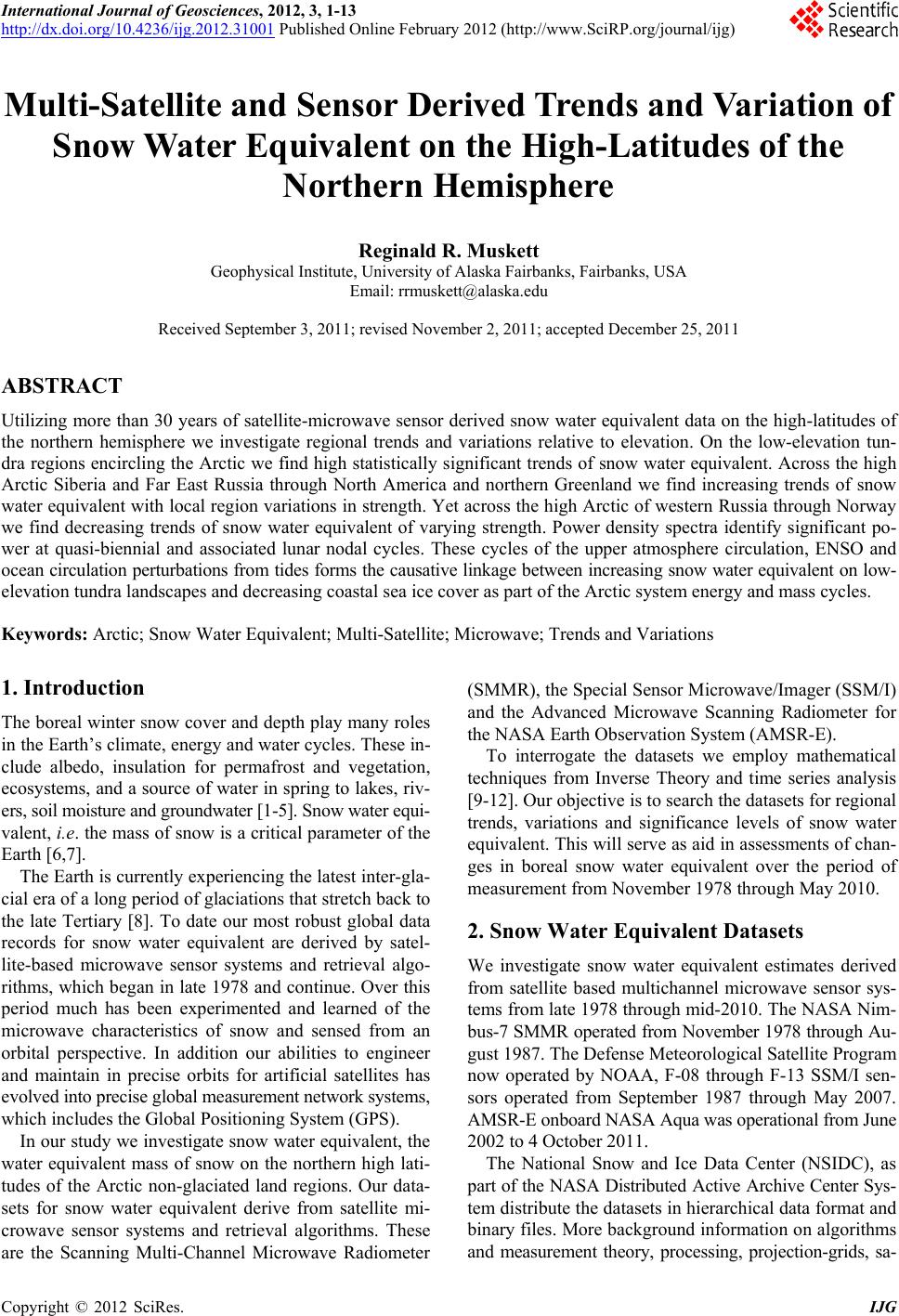
International Journal of Geosciences, 2012, 3, 1-13
http://dx.doi.org/10.4236/ijg.2012.31001 Published Online February 2012 (http://www.SciRP.org/journal/ijg)
Multi-Satellite and Sensor Derived Tr ends and Variation of
Snow Water Equivalent on the High-Latitudes of the
Northern Hemisphere
Reginald R. Muskett
Geophysical Institute, University of Alaska Fairbanks, Fairbanks, USA
Received September 3, 2011; revised November 2, 2011; accepted December 25, 2011
ABSTRACT
Utilizing more than 30 years of satellite-microwave sensor derived snow water equivalent data on the high-latitu des of
the northern hemisphere we investigate regional trends and variations relative to elevation. On the low-elevation tun-
dra regions encircling the Arctic we find high statistically significant trends of snow water equivalent. Across the high
Arctic Siberia and Far East Russia through North America and northern Greenland we find increasing trends of snow
water equivalent with local region variations in strength. Yet across the high Arctic of western Russia through Norway
we find decreasing trends of snow water equivalent of varying strength. Power density spectra identify significant po-
wer at quasi-biennial and associated lunar nodal cycles. These cycles of the upper atmosphere circulation, ENSO and
ocean circulation perturbations from tides forms the causative linkage between in creasing snow water equivalent on low-
elevation tundra landscapes and decreasing coastal sea ice cover as part of the Arctic system energy and mass cycles.
Keywords: Arctic; Snow Water Equivalent; Multi-Satellite; Microwave; Trends and Variations
1. Introduction
The boreal winter snow cover and depth play many roles
in the Earth’s climate, energy and water cycles. These in-
clude albedo, insulation for permafrost and vegetation,
ecosystems, and a source of water in spring to lakes, riv-
ers, soil moisture and groundwater [1-5]. Snow water equi -
valent, i.e. the mass of snow is a critical parameter of the
Earth [6,7].
The Earth is currently exp eriencing the latest inter-g la-
cial era of a long period of glaciations that stretch back to
the late Tertiary [8]. To date our most robust global data
records for snow water equivalent are derived by satel-
lite-based microwave sensor systems and retrieval algo-
rithms, which began in late 1978 and con tinue. Over this
period much has been experimented and learned of the
microwave characteristics of snow and sensed from an
orbital perspective. In addition our abilities to engineer
and maintain in precise orbits for artificial satellites has
evolved into precise global measurem ent network systems,
which includes the Global Positioning System (GPS).
In our study we inve stigate snow water equivalent, the
water equivalent mass of snow on the northern high lati-
tudes of the Arctic non-glaciated land regions. Our data-
sets for snow water equivalent derive from satellite mi-
crowave sensor systems and retrieval algorithms. These
are the Scanning Multi-Channel Microwave Radiometer
(SMMR), the Special Sensor Microwave/Imager (SSM/I)
and the Advanced Microwave Scanning Radiometer for
the NASA Earth Observation System (AMSR-E).
To interrogate the datasets we employ mathematical
techniques from Inverse Theory and time series analysis
[9-12]. Our objective is to search the datasets for regional
trends, variations and significance levels of snow water
equivalent. This will serve as aid in assessments of chan-
ges in boreal snow water equivalent over the period of
measurement from November 1978 through May 2010.
2. Snow Water Equivalent Datasets
We investigate snow water equivalent estimates derived
from satellite based multichannel microwave sensor sys-
tems from late 1978 through mid- 2010. The NA SA Nim-
bus-7 SMMR operated from November 1978 through Au-
gust 1987. The Defen se Meteorological Satellite Program
now operated by NOAA, F-08 through F-13 SSM/I sen-
sors operated from September 1987 through May 2007.
AMSR-E onboard NASA Aqua was operati onal from June
2002 to 4 October 2011.
The National Snow and Ice Data Center (NSIDC), as
part of the NASA Distributed Active Archive Center Sys-
tem distribute the datasets in hierarchical data format and
binary files. More background information on algorithms
and measurement theory, processing, projection-grids, sa-
C
opyright © 2012 SciRes. IJG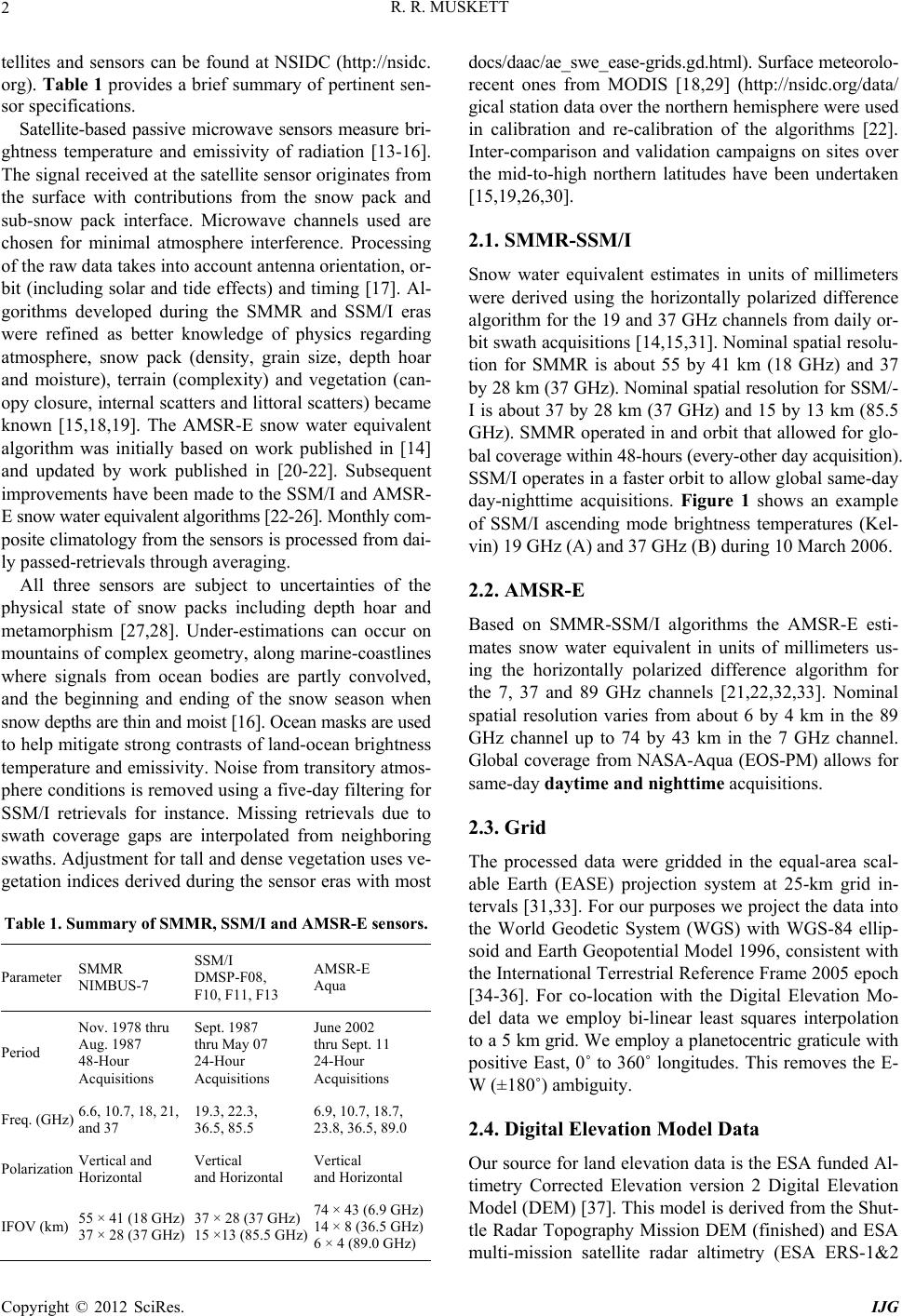

R. R. MUSKETT 2
tellites and sensors can be found at NSIDC (http://nsidc.
org). Table 1 provides a brief summary of pertinen t sen-
sor specifications.
Satellite-based passive microwave sensors measure bri-
ghtness temperature and emissivity of radiation [13-16].
The signal received at the satellite sensor originates from
the surface with contributions from the snow pack and
sub-snow pack interface. Microwave channels used are
chosen for minimal atmosphere interference. Processing
of the raw data takes into account antenna orientatio n, or-
bit (including solar and tide effects) and timing [17]. Al-
gorithms developed during the SMMR and SSM/I eras
were refined as better knowledge of physics regarding
atmosphere, snow pack (density, grain size, depth hoar
and moisture), terrain (complexity) and vegetation (can-
opy closure, internal scatters and littoral scatters) became
known [15,18,19]. The AMSR-E snow water equivalent
algorithm was initially based on work published in [14]
and updated by work published in [20-22]. Subsequent
improvements have been made to the SSM/I and AMSR-
E snow water equivalent algorithms [22-26]. Monthly com-
posite climatology from the sensors is processed from dai-
ly passed-retrievals through averaging.
All three sensors are subject to uncertainties of the
physical state of snow packs including depth hoar and
metamorphism [27,28]. Under-estimations can occur on
mountains of complex geometry, along marine-coastlines
where signals from ocean bodies are partly convolved,
and the beginning and ending of the snow season when
snow depths are thin and moist [16]. Ocean masks are used
to help mitigate strong contrasts of land-ocean brightness
temperature and emissivity. Noise from transitory atmos-
phere conditions is removed using a five-day filtering fo r
SSM/I retrievals for instance. Missing retrievals due to
swath coverage gaps are interpolated from neighboring
swaths. Adjustment for tall and dense vegetation uses ve-
getation indices derived during the sensor eras with most
Table 1. Summary of SMMR, SSM/I and AMSR-E sensors.
Parameter SMMR
NIMBUS-7
SSM/I
DMSP-F08,
F10, F11, F13
AMSR-E
Aqua
Period
Nov. 1978 thru
Aug. 1987
48-Hour
Acquisitions
Sept. 1987
thru May 07
24-Hour
Acquisitions
June 2002
thru Sept. 11
24-Hour
Acquisitions
Freq. (GHz) 6.6, 10.7, 18, 21,
and 37 19.3, 22.3, 36.5, 85.5 6.9, 10.7, 18.7, 23.8, 36.5, 89.0
Polarization Vertical and
Horizontal Vertical and Horizontal Vertical and Horizontal
IFOV (km) 55 × 41 (18 GHz)
37 × 28 (37 GHz) 37 × 28 (37 GHz) 15 ×13 (85.5 GHz)
74 × 43 (6.9 GHz)
14 × 8 (36.5 GHz)
6 × 4 (89.0 GHz)
docs/daac/ae_swe_ease-grids.gd.html). Surface meteorolo-
recent ones from MODIS [18,29] (http://nsidc.org/data/
gical station data over the northern hemisphere were used
in calibration and re-calibration of the algorithms [22].
Inter-comparison and validation campaigns on sites over
the mid-to-high northern latitudes have been undertaken
[15,19,26,30].
2.1. SMMR-SSM/I
Snow water equivalent estimates in units of millimeters
were derived using the horizontally polarized difference
algorithm for the 19 and 37 GHz channels from daily or-
bit swath acquisitions [14,15 ,31]. Nominal spatial resolu-
tion for SMMR is about 55 by 41 km (18 GHz) and 37
by 28 km (37 GHz). Nominal spatial resolution for SSM/-
I is about 37 by 28 km (37 GHz) and 15 by 13 km (85.5
GHz). SMMR operated in and orbit that allowed fo r glo-
bal coverage within 48-hours (every-other day acquisition).
SSM/I operates in a faster orbit to allow global same-day
day-nighttime acquisitions. Figure 1 shows an example
of SSM/I ascending mode brightness temperatures (Kel-
vin) 19 GHz (A) and 37 GHz (B) during 10 March 2006.
2.2. AMSR-E
Based on SMMR-SSM/I algorithms the AMSR-E esti-
mates snow water equivalent in units of millimeters us-
ing the horizontally polarized difference algorithm for
the 7, 37 and 89 GHz channels [21,22,32,33]. Nominal
spatial resolution varies from about 6 by 4 km in the 89
GHz channel up to 74 by 43 km in the 7 GHz channel.
Global coverage from NASA-Aqua (EOS-PM) allows for
same-day daytime and nighttime acquisitions.
2.3. Grid
The processed data were gridded in the equal-area scal-
able Earth (EASE) projection system at 25-km grid in-
tervals [31,33]. For our purposes we project the data into
the World Geodetic System (WGS) with WGS-84 ellip-
soid and Earth Geopotential Mod el 1996, consistent with
the International Terrestrial Reference Frame 2005 epoch
[34-36]. For co-location with the Digital Elevation Mo-
del data we employ bi-linear least squares interpolation
to a 5 km grid. We employ a planetocentric graticule with
positive East, 0˚ to 360˚ longitudes. This removes the E-
W (±180˚) ambiguity.
2.4. Digital Elevation Model Data
Our source for land elev ation data is the ESA funded Al-
timetry Corrected Elevation version 2 Digital Elevation
Model (DEM) [37]. This model is derived from the Shut-
tle Radar Topography Mission DEM (finished) and ESA
multi-mission satellite radar altimetry (ESA ERS-1&2

R. R. MUSKETT 3
Figure 1. SSM/I 19 GHz (a) and 37 GHz (b) brightness temperature (Kelvin) measured on 10 March 2006 (ascending mode)
used in the algorithm for snow water equivalent retrieval.
and Envisat) [38]. We use the 15-degree tiles, 3-arc sec-
ond posting, reference in the EGM96 WGS84 system, con-
sistent with the International Terrestrial Reference Frame
2005. For co-location matching with the snow water equi-
valent data we employ bi-linear least squares interpola-
tion (up- sampling) t o a 5 km grid.
3. Methodology
Our methodology utilizes mathematical techniques from
Inverse Theory through the investigation of time series
[9-12]. These we employ to derive least squares trends,
analysis of variations, significance levels and error.
It has long been known that topography plays impor-
tant physical roles in influencing the magnitude of pre-
cipitation, i.e. the orographic lift by terrain elevation. It
has also long been known that our satellite microwave
sensors perform with less accuracy on regions of com-
plex terrain due to slope-aspect and the limitations from
the instantaneous field of view of the sensors.
For these reasons we apply position co-location of the
snow water equivalent data with the DEM. Since our d a-
tasets are processed to have matching earth-centered grids
sorting and identifying same-location elevation with snow
water equivalent can be done efficien tly with Linux/UNIX
tools and shell scripting for batch processing. Figure 2
shows the DEM (A) and an example of snow water equi-
valent with same grid and geolocations over the Arctic.
The snow water equivalent data are for 3 March 2006.
With co-located elevation-snow water equivalent we
then extract the data filling the region beginning at 65˚N
latitude. From these we derive the 65˚N region monthly
means, standard deviations and standard errors. At this
point we then derive calibration factors of the regional-
ized monthly time series SMMR, SSM/I and AMSR-E
snow water equivalents using least squares techniques to
mitigate bias offsets of the data groups. We then apply the
calibration factors back to the 65˚N datasets using sea-
sonal sinusoids to prop ortion the calibrations by month.
Having mitigated bias offsets of the data groups we
now have a calibrated and consistent dataset covering the
non-glaciated land region from 65˚N and higher. To in-
vestigate the regional trends and variations we develop
extraction regions of interest. Figure 2(c) shows our ex-
traction region on the Arctic and the underlying DEM
with elevations in the range from 0 to 100 m. These co-
ver the Arctic Coastal Plain of Alaska and the lower Le-
na watershed for instance. Figure 2(d) gives an example
of the calibrated and co-located snow water equivalent
data in the elevation range from 0 to 100 m, 3 March 2006.
From these we derive the mean, standard deviation and
standard error of snow water equivalent and then derive
the least squares trends, p-values and significance levels.
Figure 3 shows the regionalized mean snow water equi-
valent time series in the elev ation range from 0 to 100 m,
non-calibrated (a) and calibrated (b). In Figure 3(a) we
denote the satellite-era sensors by color: Red diamonds
denote SMMR, Blue squares denote SMM/I and Green
triangles denote AMSR-E. The very obvious bias offsets
of all three are evident. Th is we can understand is mostly
a function of averaging: mostly temporal averaging from
the differing orbits from SMMR to SSM/I and spatial

R. R. MUSKETT 4
Figure 2. 65˚N region of interest for snow water equivalent (SWE) investigation. (a) ESA funded Altimetry Corrected Eleva-
tion Digital Elevation Model version 2; (b) SSM/I snow water equivalent on 3 March 2006; (c) Elevations in the range of 0 to
100 m and sub-regions referenced in Table 2 and Figure 6; (d) Elevation co-located SWE on 3 March 2006. Grey color cor-
responds to no data.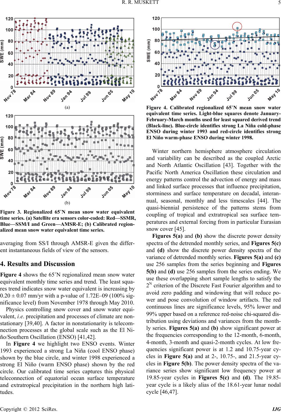

R. R. MUSKETT 5
(a)
(b)
Figure 3. Regionalized 65˚N mean snow water equivalent
time series. (a) Satellite era sensors color-coded: Red—SSMR,
Blue—SSM/I and Green—AMSR-E; (b) Calibrated region-
alized mean snow water equivalent time series.
averaging from SS/I through AMSR-E given the differ-
ent instantaneous fields of view of the sensors.
4. Results and Discussion
Figure 4 shows the 65˚N regionalized mean snow water
equivalent monthly time series and trend. The least squa-
res trend indicates snow water equivalent is increasing by
0.20 ± 0.07 mm/yr with a p-value of 1.72E–09 (100% sig-
nificance level) fro m No vember 1978 through May 2010.
Physics controlling snow cover and snow water equi-
valent, i.e. precipitation and processes of climate are non-
stationary [39,40]. A factor in nonstationa rity is telecom-
nection processes at the global scale such as the El Ni-
ño/Southern Oscillation (ENSO) [41,42].
In Figure 4 we highlight two ENSO events. Winter
1993 experienced a strong La Niña (cool ENSO phase)
shown by the blue circle, and winter 1998 experienced a
strong El Niño (warm ENSO phase) shown by the red
circle. Our calibrated time series captures this physical
teleconnection of equatorial ocean surface temperature
and extratropical precipitation in the northern high lati-
tudes.
Figure 4. Calibrated regionalized 65˚N mean snow water
equivalent time series. Light-blue squares denote January-
February-March months used for least squared derive d trend
(Black-line). Blue-circle identifies strong La Niña cold-phase
ENSO during winter 1993 and red-circle identifies strong
El Niño warm-phase ENSO during winte r 1998.
Winter northern hemisphere atmosphere circulation
and variability can be described as the coupled Arctic
and North Atlantic Oscillation [43]. Together with the
Pacific North America Oscillation these circulation and
energy patterns control the advection of energy and mass
and linked surface processes that influence precipitation,
storminess and surface temperature on decadal, interan-
nual, seasonal, monthly and less timescales [44]. The
quasi-biennial persistence of the patterns stems from
coupling of tropical and extratropical sea surface tem-
peratures and external forcing from in particular Eurasian
snow cover [45 ].
Figures 5(a) and (b) show the discrete power density
spectra of the detrended monthly series, and Figures 5(c)
and (d) show the discrete power density spectra of the
variance of detrended monthly series. Figures 5(a) and (c)
use 256 samples from the series beginning and Figures
5(b) and (d) use 256 samples from the series ending. We
use these overlapping short sample lengths to satisfy the
2N criterion of the Discrete Fast Fourier algorithm and to
avoid zero padding and windowing that will reduce po-
wer and pose convolution of window artifacts. The red
continuous lines are significance levels, 95% lower and
99 % upper based on a reference red-noise chi-squared dis-
tribution using deviations and variances from the month-
ly series. Figures 5(a) and (b) show sign ificant power at
the frequencies corresponding to the 12-month, 6-month,
4-month, 3-month and quasi-2-month cycles. At low fre-
quencies significant power is at 1.2 and 10.75-year cy-
cles in Figure 5(a) and at 2-, 10.75-, and 21.5-year cy-
cles in Figure 5(b). The power density spectra of the va-
riance series show significant low frequency power at
19.85-year cycles in Figures 5(c) and (d). The 19.85-
year cycle is a likely alias of the 18.61-year lunar nodal
cycle [46,47].

R. R. MUSKETT 6
Figure 5. Power density spectra (dB) of the calibrated regionalized 65˚N mean snow water equivalent and variance time se-
ries. (a-b) Power density spectra of 256 samples from series beginning, (a) and series ending, (b) are shown with reference
red-noise spectra at 95% significance (lower red line) and 99% significance (upper red line). (c) and (d) Power density spec-
tra of 256 samples from the variance series beginning, (c) and variance series ending, (d) are show with reference red-noise
spectra at 95% significance (lower red line) and 99% significance (upper red line).
Figure 6 shows 22 sub-region regionalized mean snow
water equivalent monthly time series and trends (Table 2)
on the northern hemisphere distributed clock-wise from
10˚E through 10˚W (Figure 2(c)). The time series verti-
cal axis is the same for all the plots. Northwest Europe
and Russia (Figure 6 and Table 2 A through E) have de-
creasing trends of snow water equivalent. Northern Si-
beria, Far East Russia and North America and Greenland
(Figure 6 and Table 2 F through V) all show increasing
trends. All have very low P-Values indicating high sig-
nificance over the period of measurement.
Figure 6(J), the Arctic Coastal Plain of Alaska shows
mean snow water equivalent values during winter 1989
were exceptionally large. Precipitation records for 1989
at Barrow, Alaska corroborate this result [48].
The mean snow water equivalent varies over all the
regions. Interestingly the largest magnitudes of regional
mean snow water equivalent occur across northern Sibe-
ria. Contrasting to this the smallest magnitudes of regio-
nal mean snow water equivalent occur across eastern North
America and Greenland.
Our regionalized trends show statistically significant
increasing snow water equivalent on low-elevation tun-
dra landscapes from northern Eurasia through North Ame-
rica and Greenland. On low-elevation tundra landscapes
fr om northern Norway through northwest Russia there are
statistically significant decreasing snow water equivalent.
These indicate a likely influence from the Atlantic inflow
and perturbation by the North Atlantic Oscillation on the
regional snow water equivalent trends [46].
Our analysis of the power density spectra has identi-
fied significant power at quasi-biennial and associated
lunar nodal cycles. The quasi-biennial (upper atmosphere
circulation and ENSO) and lunar nodal cycles (ocean cir-
culation perturbations from tides) forms the causative lin-
kage between increasing snow water equivalent on low-
elevation tundra landscapes and decreasing coastal sea
ice cover as a subsystem of the Arctic system energy and
mass cycles.
5. Conclusions
We investigate the more than 30-year record of multi-sa-
tellite and multi-microwave sensors derived snow water
equivalent on the high-latitudes of the northern hemi-
sphere land regions. We accomplish this thro ugh applica-
tion of Inverse Theory. This includes least squares cali-
br ation of the sensor snow water equivalent retrievals. We

R. R. MUSKETT 7

R. R. MUSKETT 8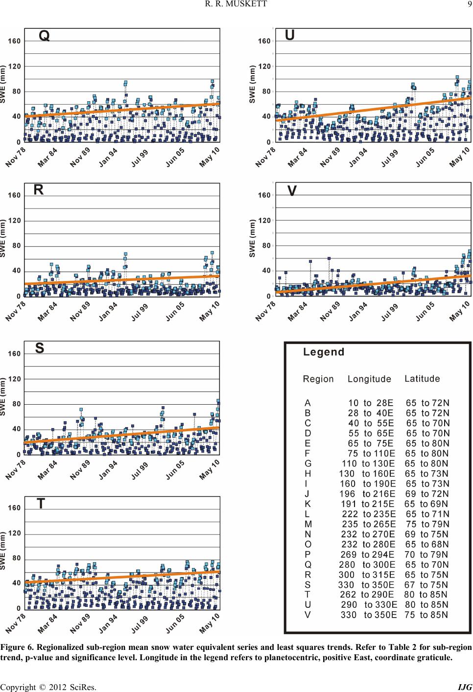

R. R. MUSKETT 9
Fi gure 6. Regionalized sub-region mean snow water equivalent series and least squares trends. Refer to Table 2 for sub-region
trend, p-value and significance level. Longitude in the le ge nd re fers to planetocentric, positive East, coordinate graticule.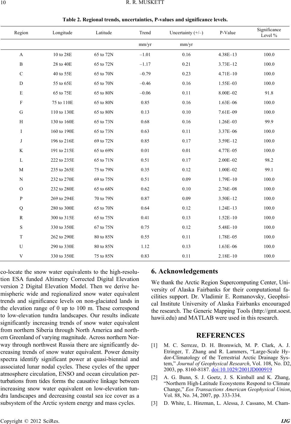

R. R. MUSKETT 10
Table 2. Regional trends, uncertainties, P-values and significance levels.
Region Longitude Latitude Trend Uncertainty (+/–)P-Value
Significance
Level %
mm/yr mm/yr
A 10 to 28E 65 to 72N –1.01 0.16 4.38E–13 100.0
B 28 to 40E 65 to 72N –1.17 0.21 3.73E–12 100.0
C 40 to 55E 65 to 70N –0.79 0.23 4.71E–10 100.0
D 55 to 65E 65 to 70N –0.46 0.16 1.55E–03 100.0
E 65 to 75E 65 to 80N –0.06 0.11 8.00E–02 91.8
F 75 to 110E 65 to 80N 0.85 0.16 1.63E–06 100.0
G 110 to 130E 65 to 80N 0.13 0.10 7.61E–09 100.0
H 130 to 160E 65 to 73N 0.68 0.16 1.26E–03 99.9
I 160 to 190E 65 to 73N 0.63 0.11 3.37E–06 100.0
J 196 to 216E 69 to 72N 0.85 0.17 3.59E–12 100.0
K 191 to 215E 65 to 69N 0.01 0.01 4.77E–05 100.0
L 222 to 235E 65 to 71N 0.51 0.17 2.00E–02 98.2
M 235 to 265E 75 to 79N 0.35 0.12 1.00E– 02 99.1
N 232 to 270E 69 to 75N 0.51 0.09 1.79E–10 100.0
O 232 to 280E 65 to 68N 0.62 0.10 2.76E–08 100.0
P 269 to 294E 70 to 79N 0.87 0.09 3.50E–12 100.0
Q 280 to 300E 65 to 70N 0.64 0.12 1.24E–13 100.0
R 300 to 315E 65 to 75N 0.41 0.13 1.52E–10 100.0
S 330 to 350E 67 to 75N 0.75 0.12 5.48E–10 100.0
T 262 to 290E 80 to 85N 0.55 0.11 1.78E–05 100.0
U 290 to 330E 80 to 85N 1.12 0.13 1.63E–06 100.0
V 330 to 350E 75 to 85N 0.83 0.11 2.18E–10 100.0
co-locate the snow water equivalents to the high-resolu-
tion ESA funded Altimetry Corrected Digital Elevation
version 2 Digital Elevation Model. Then we derive he-
mispheric wide and regionalized snow water equivalent
trends and significance levels on non-glaciated lands in
the elevation range of 0 up to 100 m. These correspond
to low-elevation tundra landscapes. Our results indicate
significantly increasing trends of snow water equivalent
from northern Siberia through North America and north-
ern Greenland of varying magnitude. Across nort hern No r-
way through northwest Russia there are significantly de-
creasing trends of snow water equivalent. Power density
spectra identify significant power at quasi-biennial and
associated lunar nodal cycles. These cycles of the upper
atmosphere circulation, ENSO and ocean circulation per-
turbations from tides forms the causative linkage between
increasing snow water equivalent on low-elevation tun-
dra landscapes and decreasing coastal sea ice cover as a
subsystem of the Arctic system energy and mass cycles.
6. Acknowledgements
We thank the Arctic Region Supercomputing Center, Uni-
versity of Alaska Fairbanks for their computational fa-
cilities support. Dr. Vladimir E. Romanovsky, Geophsi-
cal Institute University of Alaska Fairbanks encouraged
the research. The Generic Mapping Tools (http://gmt.soest.
hawii.edu) and MATLAB were used in this research.
REFERENCES
[1] M. C. Serreze, D. H. Bromwich, M. P. Clark, A. J.
Etringer, T. Zhang and R. Lammers, “Large-Scale Hy-
dor-Climatology of the Terrestrial Arctic Drainage Sys-
tem,” Journal of Geophysical Research, Vol. 108, No. D2,
2003, pp. 8160-8187. doi:10.1029/2001JD000919
[2] A. G. Bunn, S. J. Goetz, J. S. Kimball and K. Zhang,
“Northern High-Latitude Ecosystems Respond to Climate
Change,” Eos Transactions American Geophysical Union,
Vol. 88, No. 34, 2007, pp. 333-334.
[3] D. White, L. Hinzman, L. Alessa, J. Cassano, M. Cham-

R. R. MUSKETT 11
bers, K. Falkner, J. Francis, W. J. Gutowski Jr., M. Hol-
land, R. M. Holmes, H. Huntington, D. Kane, A. Kliskey,
C. Lee, J. McClelland, B. Peterson, T. S. Rupp, F. Stra-
neo, M. Steele, R. Woodgate, D. Yang, K. Yoshikawa
and T. Zhang, “The Arctic Freshwater System: Changes
and Impacts,” Journal of Geophysical Research, Vol. 112,
2007, G04S54. doi:10.1029/2006JG000353
[4] U. S. Bhatt, D. A. Walker, M. K. Raynolds, J. C. Comiso,
H. E. Epstein, G. Jia, R. Gens, J. E. Pinzon, C. J. Tucker,
C. E. Tweedie and P. J. Webber, “Circumpolar Arctic
Tundra Vegetation Change Is Linked to Sea Ice Decline,”
Earth Interactions, Vol. 14, No. 8, 2010, pp. 1-20,
doi:10.1175/2010EI315.1
[5] G. Grosse, S. Marchenko, V. Romanovsky, K. P. Wick-
land, N. French, M. Waldrop, L. Bourgeau-Chavez, R.
Striegl, J. Harden, M. Turetsky, A. D. McGuire, P. Camill,
C. Tarnocai, S. Frolking, E. Schuur and T. Jorgenson,
“Vulnerability of High Latitude Soil Organic Carbon in
North America to Disturbance,” Journal of Geophysical
Research, Vol. 116, 2011, G00K06.
doi:10.1029/2010JG001507
[6] R. E. Dickinson, “Land Surface Processes and Climate --
Surface Albedos and Energy Balance,” In: B. Saltzman,
Ed., Advances in Geophysics, Theory of Climate, Vol. 25,
Academic Press, New York, 1983.
[7] B. F. Chao, W. P. O’Connor, A. T. C. Chang, D. K. Hall
and J. L. Foster, “Snow Load Effect on the Earth’s Rota-
tion and Gravitational Field, 1979-1985,” Journal of Geo-
physical Research, Vol. 92, No. B9, 1987, pp. 9415-9422.
doi:10.1029/JB092iB09p09415
[8] C. K. Seyfert and L. A. Sirkin, “Earth History and Plate
Tectonics: An Introduction to Historical Geology,” 2nd
Edition, Harper & Row Publishers, Inc., New York, 1979.
[9] P. J. Brockwell and R. A. Davis, “Time Series: Theory
and Methods,” 2nd Edition, Springer-Verlag, New York,
1991. doi:10.1007/978-1-4419-0320-4
[10] P. R. Bevington and D. K. Robinson, “Data Reduction
and Error Analysis for the Physical Sciences,” 2nd Edi-
tion, McGraw-Hill Inc., New York, 1992.
[11] J. A. Scales, M. L. Smith and S. Treitel, “Introductory
Inverse Theory,” Samizdat Press, Golden, 2001.
[12] G. J. Borradaile, “Statistics of Earth Science Data: Their
Distribution in Space, Time and Orientation,” Springer-
Verlag, Berlin, 2003.
[13] K. F. Kunzi, S. Patil and H. Rott, “Snow-Cover Parame-
ters Retrieved from Nimbus-7 Scanning Multichannel
Microwave Radiometer (SMMR) Data,” IEEE Transac-
tions on Geoscience and Remote Sensing, Vol. 20, No. 4,
1982, pp. 452-467. doi:10.1109/TGRS.1982.350411
[14] A. T. C. Chang, J. L. Foster and D. K. Hall, “Nimbus-7
SMMR Derived Global Snow Cover Parameters,” Annals
of Glaciology, Vol. 9, 1987, pp. 39-44.
[15] A. T. C. Chang, J. L. Foster and D. K. Hall, “Satellite
Sensor Estimates of Northern Hemisphere Snow Vol-
ume,” International Journal of Remote Sensing, Vol. 11,
No. 1, 1990, pp. 167-171.
doi:10.1080/01431169008955009
[16] L. S. Koenig and R. R. Forster, “Evaluation of Passive
Microwave Snow Water Equivalent Algorithms in the
Depth Hoar-Dominated Snowpack of the Kuparuk River
Watershed, Alaska, USA,” Remote Sensing of Environ-
ment, Vol. 93, No. 4, 2004, pp. 511-527.
doi:10.1016/j.rse.2004.08.004
[17] E. G. Njoku, “Antenna Pattern Correction Procedures for
the Scanning Multichannel Microwave Radiometer (SM-
MR),” Boundary-Layer Meteorology, Vol. 18, 1980, pp.
79-98. doi:10.1007/BF00117912
[18] A. T. C. Chang, J. L. Foster and D. K. Hall, “Effects of
Forest on the Snow Parameters Derived from Microwave
Measurements during the BOREAS Winter Field Cam-
paign,” Hydrological Processes, Vol. 10, No. 12, 1996,
pp. 1565-1574.
doi:10.1002/(SICI)1099-1085(199612)10:12<1565::AID-
HYP501>3.0.CO;2-5
[19] R. J. Armstrong and M. J. Brodzik, “Recent Northern
Hemisphere Snow Extent: A Comparison of Data from
Visible and Microwave Satellite Sensors,” Geophysical
Research Letters, Vol. 28, No. 19, 2001, pp. 3673-3676.
doi:10.1029/2000GL012556
[20] A. T. C. Chang, J. L. Foster, D. K. Hall, B. E. Goodison,
A. E. Walker and J. R. Metcalfe. “Snow Parameters De-
rived from Microwave Measurements during the BO-
REAS Winter Field Experiment,” Journal of Geophysical
Research, Vol. 102, No. D24, 1997, pp. 29663-29671.
doi:10.1029/96JD03327
[21] R. Kelly, A. Chang, L. Tsang and J. Foster, “A Prototype
AMSR-E Global Snow Area and Snow Depth Algo-
rithm,” IEEE Transactions on Geoscience and Remote
Sensing, Vol. 41, No. 2, 2003, pp. 230-242.
doi:10.1109/TGRS.2003.809118
[22] R. E. J. Kelly and A. T. C. Chang, “Development of a
Passive Microwave Global Snow Depth Retrieval Algo-
rithm for Special Sensor Microwave Imagery (SSM/I)
and Advanced Microwave Scanning Radiometer-EOS
(AMSR-E) Data,” Radio Science, Vol. 38, No. 4, 2003,
pp. 1-11. doi:10.1029/2002RS002648
[23] R. J. Kelly and J. L. Foster, “The AMSR-E Snow Water
Equivalent Product: Status and Future Development,”
American Geophysical Union, Fal l Meeting 2005, Abstract
#C21C-1134, 2005.
[24] R. E. J. Kelly, J. L. Foster and D. K. Hall, “The AMSR-E
Snow Water Equivalent Product: Algorithm Development
and Progress in Product Validation,” Proceedings of the
28th General Assembly of the Union of International Ra-
dio Science, New Delhi, 23-29 October 2005.
[25] S. Biancamaria, N. Mognard, A. Boone, M. Grippa and E.
Josberger, “A Satellite Snow Depth Multi-Year Average
Derived from SSM/I for the High Latitude Regions,”
Remote Sensing of Environment, Vol. 112, No. 5, 2008,
pp. 2557-2568. doi:10.1016/j.rse.2007.12.002
[26] C. Derksen, P. Toose, A. Rees, L. Wang, M. English, A.
Walker and M. Sturm, “Development of a Tundra-Spe-
cific Snow Water Equivalent Retrieval Algorithm for
Satellite Passive Microwave Data,” Remote Sensing of
Environment, Vol. 114, No. 8, 2010, pp. 1699-1709.
doi:10.1016/j.rse.2010.02.019
[27] D. K. Hall, R. E. J. Kelly, G. A. Riggs, A. T. C. Chang

R. R. MUSKETT 12
and J. L. Foster, “Assessment of the Relative Accuracy of
Hemispheric-Scale Snow-Cover Maps,” Annals of Glaci-
ology, Vol. 34, 2002, pp. 24-30.
[28] J. L. Foster, C. Sun, J. P. Walker, R. Kelly, A. Chang, J.
Dong and H. Powell, “Quantifying the Uncertainty in
Passive Microwave Snow Water Equivalent Observations,”
Remote Sensing of Environment, Vol. 94, No. 2, 2005, pp.
187-203. doi:10.1016/j.rse.200409.012
[29] J. T. Pulliainen, J. Grandell and M. T. Hallikainen, “Re-
trieval of Surface Temperature in Boreal Forest Zone
from SSM/I Data,” IEEE Transactions on Geoscience
and Remote Sensing, Vol. 35, No. 5, 1997, pp. 1188-1200.
doi:10.1109/36.628786
[30] A. T. C. Chang, J. L. Foster, R. E. J. Kelly, E. G. Josber-
ger, R. L. Armstrong and N. M. Mognard, “Analysis of
Ground-Measured and Passive-Microwave-Derived Snow
Depth Variations in Midwinter across the Northern Great
Plains,” Journal of Hydormet, Vol. 6, No. 1, 2005, pp.
20-33. doi:10.1175/JHM-404.1
[31] R. J. Armstrong, M. J. Brodzik, K. Knowles and M. Sa-
voie, “Global Monthly EASE-Grid Snow Water Equiva-
lent Climatology,” National Snow and Ice Data Center,
University of Colorado Boulder, 2007.
http://nsidc.org/data/docs/daac/nsidc0271_ease_grid_swe
_climatology.gd.html
[32] A. T. C. Chang and A. Rango, “Algorithm Theoretical
Basis Document for the AMSR-E Snow Water Equivalent
Algorithm, Version 3.1,” NASA Goddard Space Flight
Center, 2000.
http://nsidc.org/data/amsre/pdfs/amsr_atbd_snow.pdf
[33] M. Tedesco, R. E. J. Kelly, J. L. Foster and A. T. C.
Chang, “AMSR-E/Aqua Monthly L3 Global Snow Water
Equivalent EASE-Grids V002,” National Snow and Ice
Data Center, University of Colorado Boulder, 2004.
http://nsidc.org/data/docs/daac/ae_swe_ease-grids.gd.htm
l.
[34] F. G. Lemoine, S. C. Kenyon, J. K. Factor, R. G. Trim-
mer, N. K. Palvis, D. S. Chinn, C. M. Cox, S. M. Klosko,
S. B. Luthcke, M. H. Torrence, Y. M. Wang, R. G. Wil-
liamson, E. C. Pavlis, R. H. Rapp and T. R. Olson, “The
Development of the Joint NASA GSFC and the National
Imagery and Mapping Agency (NIMA) Geopotential Model
EGM96,” NASA Goddard Space Flight Center, NASA/
TP-1998-206861, Maryland, 1998.
[35] National Imagery and Mapping Agency (NIMA), “De-
partment of Defense World Geodetic System 1984: Its
Definition, and Relationship with Local Geodetic Sys-
tems, TR8350.2, Third Ed., Ammendment 1,” Depart-
ment of Defense, Washington DC, 2000.
[36] Z. Altamimi, X. Collilieux, J. Legrand, B. Garayt and C.
Boucher, “ITRF2005: A New Release of the International
Terrestrial Reference Frame on Time Series of Station
Positions and Earth Orientation Parameters,” Journal of
Geophysical Research, Vol. 112, 2007, B09401.
doi:10.1029/2007JB004949
[37] P. A. M. Berry, R. G. Smith, J. A. Freeman and J. Ben-
veniste, “Towards a New Global Digital Elevation
Model,” In: M. G. Sideris, Ed., Observing Our Change
Earth, Vol. 133, Part 2, 2008, pp. 431-435.
http://tethys.eaprs.cse.dum.ac.uk
[38] R. G. Smith, P. A. M. Berry and J. Benveniste, “Repre-
sentation of Rivers and Lakes within the Forthcoming
ACE2 Global Digital Elevation Model,” ESA 2nd Space
for Hydrology Workshop, Geneva, 12-14 November 2007.
http://earth.esa.int/hydrospace07/participants/04_03/04_0
3_Smith.pdf
[39] K. E. Trenberth, “Recent Observed Interdacadal Climate
Changes in the Northern Hemisphere,” Bulletin of the
American Meteorological Society, Vol. 7, 1990, pp. 988-
993.
doi:10.1175/1520-0477(1990)071<0988:ROICCI>2.0.CO
;2
[40] G. Wang and P. Yang, “A Compound Reconstructed
Prediction Model for Nonstationary Climate Processes,”
International Journal of Climatol ogy, Vol. 25, No. 9, 2005,
pp. 1265-1277. doi:10.1002/joc.1158
[41] A. Dai and T. M. L. Wigley, “Global Patterns of ENSO-
Induced Precipitation,” Geophysical Research Letters,
Vol. 27, No. 9, 2000, pp. 1283-1286.
doi:10.1029/1999GL011140
[42] O. Timm, M. Pfeiffer and W.-C. Dullo, “Nonstationary
ENSO-Precipitation Teleconnections over the Equatorial
Indian Ocean Documented in a Coral from the Chagos
Archipelago,” Geophysical Research Letters, Vol. 32, 2005,
L02701. doi:10.1029/2004GL021738
[43] D. W. J. Thompson and J. M. Wallace, “Annular Modes
in the Extratropical Circulation. Part I: Month-to-Month
Variability,” Journal of Climate, Vol. 13, No. 5, 2000, pp.
1000-1016.
doi:10.1175/1520-0442(2000)013<1000:AMITEC>2.0.C
O;2
[44] S. B. Feldstein, “The Timescale, Power Spectra, and Cli-
mate Noise Properties of Teleconnection Patterns,” Jour-
nal of Climate, Vol. 13, No. 24, 2000, pp. 4430-4440.
[45] R. J. Allen and C. S. Zender, “The Role of Eastern Si-
berican Snow and Soild Moisture Anomalies in Quasi-
Biennial Persistence of the Arctic and North Atlantic Os-
cillations,” Journal of Geophysical Research, Vol. 116,
2011, D16125. doi:10.1029/2010JD015311
[46] H. Yndestad, “The Influence of the Lunar Nodal Cycle on
Arctic Climate,” ICES Journal of Marine Science, Vol.
63, No. 3, 2006, pp. 401-420.
[47] I. D. Haigh, M. Eliot and C. Pattiaratci, “Global Influ-
ences of the 18.61 Year Nodal Cycle and the 8.85 Year
Cycle of Lunar Perigee on High Time Levels,” Journal of
Geophysical Research, Vol. 116, 2011, C06025.
doi:10.1029/2010JC006645
[48] M. Shulski and G. Wendler, “The Climate of Alaska,”
University of Alaska Press, Fairbanks, 2007.
[49] D. Ghatak, A. Frei, G. Gong, J. Stroeve and D. Robinson,
“On the Emergence of an Arctic Amplification Signal in
Terrestrial Arctic Snow Extent,” Journal of Geophysical
Research, Vol. 115, 2010, D24105.
doi:10.1029/2010JD014007
[50] G. Wendler, M. Shulski and B. Moore, “Changes in the
Climate of the Alaskan North Slope and the Ice Concen-
tration of the Adjacent Beaufort Sea,” Theoretical and

R. R. MUSKETT 13
Applied Climatology, Vol. 99, No. 1, 2010, pp. 67-74.
doi:10.1007/s00704-009-0127-8
[51] M. C. Serreze, A. P. Barrett, A. G. Slater, R. A. Wood-
gate, K. Aagaard, R. B. Lammers, M. Steele, R. Moritz,
M. Merrdith and C. M. Lee, “The Large-Scale Freshwater
Cycle of the Arctic,” Journal of Geophysical Research,
Vol. 111, 2006, C11010. doi:10.1029/2005JC003424