Journal of Geographic Information System, 2010, 2, 93-99
doi:10.4236/jgis.2010.22014 Published Online April 2010 (http://www.SciRP.org/journal/jgis)
Remote Sensing and GIS as an Advance Space Technologies
for Rare Vegetation Monitoring in Gobustan State
National Park, Azerbaijan
Yelena M. Gambarova1, Adil Y. Gambarov2, Rustam B. Rustamov3, Maral H. Zeynalova4
1R.I.S.K. Company, Baku, Azerbaijan
2SAHIL IT Company, Baku, Azerbaijan
3Institute of Physics of the National Academy of Sciences, Baku, Azerbaijan
4Institute of Botany of the National Academy of Sciences, Baku, Azerbaijan
Abstract
This paper describes remote sensing methodologies for monitoring rare vegetation with special emphasis on
the Image Statistic Analysis for set of training samples and classification. At first 5 types of Rare Vegetation
communities were defined and the Initial classification scheme was designed on that base. After preliminary
Statistic Analysis for training samples, a modification algorithm of the classification scheme was defined:
one led us to creating a 4 class’s scheme (Final classification scheme). The different methods analysis such
as signature statistics, signature separability and scatter plots are used. According to the results, the average
separability (Transformed Divergence) is 1951.14, minimum is 1732.44 and maximum is 2000 which shows
an acceptable level of accuracy. Contingency Matrix computed on the results of the training on Final classi-
fication scheme achieves better results, in terms of overall accuracy, than the training on Initial classification
scheme.
Keywords: Remote Sensing, GIS, Seperability, Classification
1. Introduction
The vegetation is one of th e key and best instrument and
indicator for monitoring of identification of impacts of
the natural processes, environmental and ecological is-
sues. As changes in vegetation are rapid and serious due
to various human activities, it is urgent to monitor vege-
tation and their surrounding environment from physical,
biological or social viewpoints. Remote sensing is ex-
pected to provide us an efficient tool for monitoring vege-
tation environment. In particular, as considering vegeta-
tion is often characterized by a mixture of different vege-
tations, soil and water, remote sensing is expected to
delineate the relation between them.
This paper describes Remote Sensing and GIS as an
advance Space Technology for Rare Vegetation moni-
toring in Gobustan State National Park with special em-
phasis on Image Statistic Analysis for set of training
samples and classification.
Determination of the ‘best’ bands combinations in the
context of Image statistical analysis is very important.
The best band combinations will be used in accurate
classification. Methods used to select the optimum bands
combination are known as feature selection techniques.
A number of criteria can be used to categorize feature
selection techniques. As they can be classified on the
basis of whether they are graphical or statistical in nature
[1], they can also be classified into two categories based
on whether or not they use classification algorithms to
evaluate the performance of subsets. Techniques that use
the former approach are called ‘wrapper techniques’;
techniques using the latter approach are known as ‘filter
techniques’ [2].
A filter is defined as a feature selection algorithm using
a performance metric based entirely on the training data,
without reference to the classifier for which the features
are to be selected. The most widely used filter methods
are based on class separability indices. Use of this ap-
proach in the context of Image statistical analysis was
investigated in this stud y. Class Separab ility indices were
employed to determine the best band combination of
SPOT 5 image datasets.

Y. M. GAMBAROVA ET AL. 94
These indices have been extensively used by research-
ers in remote sensing for many years [3-5].
Some researchers sought to test whether some bands
had more discriminating power than others by using the
Jeffries-Matusita distance analysis technique only [3], [5]
and [6]. Other researchers, for this purpose, Divergence
Distance or Battacharrya Distance were used to measure
the separability [4 ], [5] and [7].
In our case, of the four separability indices compared,
the use of transformed measures (Transformed Diverg-
ence and the Jeffries-Matusita distance) in the Class
Separability appeared to be more powerful than other
methods. Transformed divergence and the Jeffries-Matu-
sita distance both found the best solution with the highest
classification accuracy.
2. Study Area
This study was carried out in Gobustan, located between
the southern outcrops of the Caucasus Mountain range
and the Caspian Sea, some 60 km south of the capital
Baku as in presented in the Figure 1.
The Study Area at Gobustan (covering the area of
282 km2) contains a wealth of historical and archaeo-
logical sites and is also known for its rare vegetation.
The vegetation communities in the study area repress-
ent the most ecologically important habitat. Some of
Rare Vegetation communities within the expected for
investigation area presently classified as either rare or
threatened and recommended for inclusion into the Nat-
ional Red Book. The importance of this habitat type is
one of the reasons why the Gobustan State National Park
has been proposed, so that some level of protection is
offered to this desert.
3. Data Used and Methodology
Four SPOT5 images in 2.5 m and 5 m resolutions, ac-
quired between 2004 and 2007 were used for the delinea-
tion and classification of Ra re Vegetation comm uniti es.
Figure 1. Study area.

Y. M. GAMBAROVA ET AL.95
The sampling scheme was designed to collect the rare
vegetation commun ities in Gobustan Natio nal Park study
site for combined ecological and remote sensing studies.
The Field surveys were hold in accordance with prelimi-
nary data on the spreading of rare plants in the study area.
Quadrates and plots assisted by satellite SPOT 5 imagery
have provided information on habitat types and status.
Because GPS devices provided the coordinates for ground-
reference data during fieldwork, the sample plots were
accurately linked to SPOT imagery. Every plot was reg-
istered with GPS Garmin device to allow further inte-
gration with spatial data in GIS and image processing
systems (Figure 2).
4. Definition of the Initial Classification
Scheme
Classification process involves three steps: 1) training, 2)
classification and 3) output and validation.
In the training stage Initially 5 types of Rare Vegeta-
tion communities were defined that—according to ecolo-
gists’ opinion—are indicators of climate and ecosystem
properties in the region being studied. Below the Latin
names of them are presented (Table 1). At first, these
sites were geolocated, then using GIS procedures the
areas of location of these vegetation communities were
determined for extraction of samples for the classifier
training and testing .
The set of training samples was tested for Representat-
iveness and Separability based on their calculated statis-
tical parameters. There are the tests to perform that can
help determine whether the set of training samples are a
true representation of the pixels to be classified for each
class.
It is important that the training areas be representative
of the full variability of spectral response in that class.
Author [8] recommends that a minimum of 10 n to 100 n
pixels be part of training areas, where n is the number of
spectral bands. Hence, in our case, with SPOT data, the
requirement is for roughly 30 to 300 pixels per class.
4.1. Image Statistical Analysis: The Initial
Classification Scheme
Once the training areas are selected, different methods
are used for testing purposes such as histograms, separa-
bility, signature statistics and scatter plots.
The visualization technique in feature space allows es-
timating range of the correlation of training samples:
thereto, for each of the class from the training data was
estimated of Minimum and Maximum values on each
band used and created three-dimensional parallelepiped
in the feature space. Or, another way is to define a three-
dimensional ellipsoid, estimated of Mean ± Standard
deviations valu es on each band used.
Figure 2. Interpretation of SPOT image and field survey.

Y. M. GAMBAROVA ET AL. 96
Table 1. Rare vegetation communities. Initial classification
scheme.
Class The name of vegetation communities
Class 1 Alhagi pseudoalhagi
Class 2 Salsola Nodulosa/Artemisia Lerchiana
Class 3 Salsola Nodulosa/Salsola Dendroides
Class 4 Tamarix
Class 5 Suaeda Dendroides
4.2. Compare Ellipses
We can view graphs of these statis tics for compare cla s ses .
The graphs display as sets of ellipses in a Feature Space
image. Each ellipse is based on the mean and standard
deviation of one class. The color is used as the color for
the class in the visualization functions, ellipses, etc. The
ellipses are presented with the color regarding each class
as is shown in table below.
Class Number The name of vegetation communities Color
Class 1 Alhagi pseudoalhagi
Class 2 Salsola Nodulosa/Artemisia Lerchiana
Class 3 Salsola Nodulosa/Salsola Dendroides
Class 4 Tamarix
Class 5 Suaeda Dendroides
By comparing the ellipses for different classes for a
one band pair, it is easy to see if the training set repre-
sents similar groups of pixels by seeing where the ellip-
ses overlap on the Feature Space image (Figure 3). As
shown in Figure 3, the ellipses are overlapped, that me ans
the set of training samples (excepting class Alhagi pseu-
doalhagi) represent similar pixels, which is not desirable
for classification.
4.3. Class Separability: Initial Classification
Scheme
Separability can be evaluated for any combination of
bands that is used in the classification, enabling you to
rule out any bands that are not useful in th e results of the
classification. These distances used to determine the b est
results to use in the classification. If the spectral distance
between two samples is not significant for any pair of
bands, then signatures may not be distinct enough to pro-
duce a successful classification. We evaluated the Average
and Minimum Separability on all formulas for the band
set. The Best Minimum and Best Average Separability
values present in Table 2.
Figure 3. Band combination. Sets of ellipses in the feature
space image.

Y. M. GAMBAROVA ET AL.97
Although for completeness we presented all four
methods for calculating separability (Table 3), generally
two different formulas were used: Transformed Diver-
gence (TD) and Jeffries-Matusita distance (JM).
Transformed Divergence and the Jefferies-Matusita
distance both found the best solution with the highest
classification accuracy.
According [1] both TD and JM have upper and lower
bounds:
Transformed D i vergence is between 0 and 2000
Jefferies-Matusita Distance is between 0 and 1414
As a general rule, if the result is greater than 1900,
then classes can be separated. Between 1700 and 1900
the separation is fairly good. Below 1700, the separation
is poor [1].
Analyzing the results shown in Table 2 we can unam-
biguously concluded that the classes are poor separable
(Class separability values greatly lower bounds) and these
training samples could not used for accuracy classifica-
tion. For confirmation this conclusion a Contingency Ma-
trix was calculated (Table 3).
4.4. Contingency Matrix: Initial Classification
Scheme
Contingency Matrix do a quick classification of the pixels
in a set of training samples to see what percentag e of the
sample pixels are actually classified as expected [9].
In theory, each training sample would be composed
primarily of pixels that belong to its co rresponding class.
Practically, as are shown in Table 4 , only all pixels fro m
Class 1—Alhagi pseudoalhag—classified correctly (ass-
igned to its class). The overall accuracy was calculated
by summing the main diagonal elements of the Contin-
gency matrix and dividing by the total number of sam-
ples.
These tests have shown that: Class 3 has completely
contained Class 2; Class 4 and Class 5 have heavily ove r-
lapped each other. These undesir able resu lts of Statistical
tests and Class Separability generated the need to per-
form any operations to improve (qualify) of Initial clas-
sification scheme. These tests pointed out to a direction
of possible modification of “Initial classification sc h eme” ,
for that an additional set of training samples was req-
uired.
5. Definition of the Final Classification
Scheme
In the during field surveys a new sites for collection
training samples was defined.
After analyzing the results it would be beneficial to
merge Class 2 (Salsola Nodulosa/Artemisia Lerchiana and
Class 3 (Salsola Nodulosa/Salsola Dendroides) into one
class:
Table 2. Best minimum and best average separability (Initial classification scheme).
Band Combination Euclidean Distance Divergence Transformed Divergence Jefferies-Matusita Distance
MIN AVE MIN AVE MIN AVE MIN AVE
1 2 3 3 36 1 99 286 1414 525 1088
1 2 3 29 2 463 527 1730 436 1043
1 3 4 425 787 1699 408 1052
2 3 3 35
2 2 29 4 472 747 1736 123 741
Table 3. Contingency matrix. Initial classification scheme.
Class Number Class 1 Class 2 Class 3 Class 4 Class 5 Row T otal
Class 1 226 0 0 0 0 226
Class 2 0 775 212 205 11 1203
Class 3 0 88 644 126 2 860
Class 4 0 352 378 471 0 1201
Class 5 0 169 115 24 176 484
Column Total 226 1384 1349 826 189 3974
Overall Accuracy = 57.6%

Y. M. GAMBAROVA ET AL. 98
(SalsolaNodulosa/ArtemisiaLerchiana_SalsolaNodulosa/
SalsolaDendroides).
The algorithm of this modification is presented (Table
4). There was received the Final classification scheme
consisted of four classes:
Having received the new set, we performed the same
statistical tests of representativeness and separability w hi ch
show the advances have come using new Final classifica-
tion scheme.
5.1. Class Separability: Final Classification
Scheme
The Class Separability on Final classification scheme was
arranged in matrix form.
We evaluated Transformed Divergence (TD) and Jeffer-
ies-Matusita Distance (JM) for every class pair and one
band combination. Then we compared these num- bers
(values) to other separability listings for other band com-
binations to determine which set of bands is the most
useful for classification.
The Table 5 and Table 6 present the Transformed
Divergence matrix and the Jefferies-Matusita Distance
separability matrix on the best band combinations.
Analyzing the numerical TD values (Table 5) we can
conclude that the separability results for training samples
on final classification scheme are good enough with the
exception of class pair 2:4. The Best Average Separabil-
ity is 1951.14, Minimum Separability is 1732.44 and
Maximum Separability is 2000. That is to say Class S epa -
rability values greater th an 1900 where ob tained for most
classes, besides for Class 1 the TD value is 2000 – upper
bound.
Also the values of the JM distance for the data set
(Table 6) are greater than the values obtaine d from Initial
scheme data (Table 2). Having acceptable levels for the
separability of the training areas, the next step is to con-
duct the classification process.
Overall, Class Separability is adequate and would pro-
vide a fairly accurate classification.
Table 4. Final classification scheme.
Class Classified Data
Class 1 Alhagi pseudoalhagi
Class 2 Salsola Nodulosa/Artemisia Lerchiana_Salsola
Nodulosa/Salsola Dendroides
Class 3 Tamarix
Class 4 Suaeda Dendroides
Table 5. Transformed divergence separability matrix for training classes.
Distance Measure: Transformed Divergence
Best Average Separability: 1951.14
Band Combination: 1_2
Signature Name Class 1 2 3 4
Alhagi pseudoalhagi 1 0 2000 2000 2000
Tamarix 2 2000 0 1975.13 1732.44
Suaeda Dendroides 3 2000 1975.13 0 1999.25
Salsola Nodulosa/Artemisia Lerchiana_Salsola
Nodulosa/Salsola Dendroides 4 2000 1732.44 1999.25 0
Table 6. Jefferies-matusita distance separability matrix for training classes.
Distance Measure: Jefferies-Matusita
Best Average Separability: 1208.63
Band Combination: 1_2_3
Signature Name Class 1 2 3 4
Alhagi pseudoalhagi 1 0 1411.5 1402.88 1367.45
Tamarix 2 1411.5 0 1255.07 1010.43
Suaeda Dendroides 3 1402.88 1255.07 0 904.43
Salsola Nodulosa/Artemisia Lerchiana_ Salsola
Nodulosa/Salsola Dendroides 4 1367.45 1010.43 904.43 0

Y. M. GAMBAROVA ET AL.99
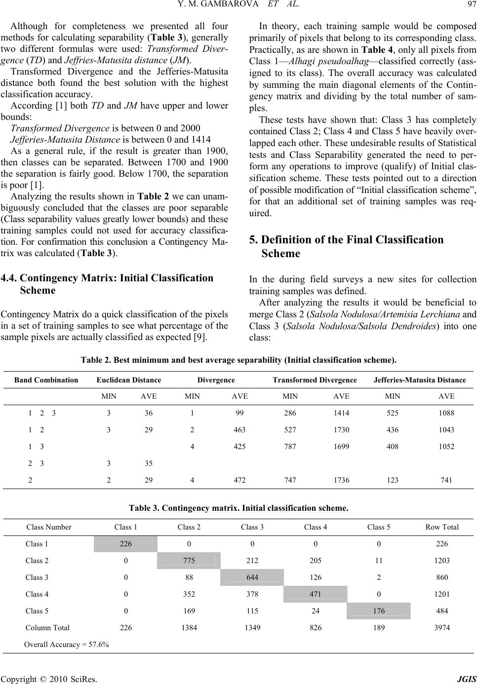
Table 7. Contingency matrix. Final classification scheme.
Classified Data Alhagi pseudoalhagiTamarix Suaeda DendroidesSalsolaNodulosa/Artemisia
Lerchiana/SalsolaNodulosa/Salsola
Dendroides
Alhagi pseudoalhagi 151 0 0 28
Tamarix 0 342 0 151
Suaeda Dendroides 1 11 65 128
SalsolaNodulosa/Artemisia
Lerchiana_SalsolaNodulosa/Salsola
Dendroides 5 20 11 462
Column Total 157 373 76 769
Overall Accuracy = 74.2%
5.2. Contingency Matrix: Final Classification
Scheme
A common method for classification accuracy assessm-
ent is through the use of the Contingency Matrix. The
Overall Accuracy is 74.2% (Table 7).
It has been found that the Contingency Matrix com-
puted on the results of the training on Final classification
scheme achieves better results, in terms of overall accu-
racy (overall accuracy = 74.2%) than the training on Ini-
tial classification scheme (overall accuracy = 57.6%).
6. Conclusions
The aim of this study was to perform the Image Statist-
ical analysis in the training stage. The number of multi-
variate statistical techniques was employed to estimate
the degree of discrimination between the classes. At
every step of the training process, values of Class Sep-
arability as represented by Transformed Divergence and
Jefferies-Matusita Distance where evaluated as a measur e
of the quality of training areas. Training areas for first
dataset (Initial classification scheme) that produced TD
coefficients lower than 1700 for either measure where
rejected (Table 2 and Table 3).
The Image Statistical analysis of Final classification
scheme (modified scheme) have shown the advances of
new Final classification scheme and determined the best
combinations of bands for separating the classes from
each other (Table 6 and Table 7).
The accuracy in this classification suggested that this
strategy for the selection of training samples, modifica-
tion of classification scheme used were importance to
perform better classification result.
7. Acknowledgements
This work was supported by the Planet Action and the
Idea Wild non-profit organizations for their support by
donating satellite images, GIS software and equipment,
which provided recourses for the research that led to this
paper.
8. References
[1] J. R. Jensen, “Introductory Digital Image Processing: A
Remote Sensing Perspective,” Prentice Hall, London,
1996.
[2] T. Kavzoglu and P. Mather, “The Role of Feature Selec-
tion in Artificial Neural Network Applications,” Interna-
tional Journal Remote Sensi ng, Vol. 23, No. 15, 2002, pp.
2919- 2937.
[3] I. L. Thomas, V. M. Benning and N. P. Ching, “Classifi-
cation of Remotely Sensed Images,” Adam Hilger, Lon-
don, 1987.
[4] L. V. Dutra and R. I. Huber, “Feature Extraction and
Selection for ERS-1/2 in SAR Classification,” Interna-
tional Journal of Remote Sensing, Vol. 20, No. 5, 1999,
pp. 993-1016.
[5] B. M. Tso and P. M. Mather, “Crop Discrimination Using
Multi-Temporal SAR Imagery,” International Journal of
Remote Sensing, Vol. 20, No. 12, 1999, pp. 2443-2460.
[6] O. Mutanga, I. Riyad, A. Fethi and K. Lalit, “Imaging
Spectroscopy (Hyperspectral Remote Sensing) in South-
ern Africa: An Overview,” South African Journal of Sci-
ence, Vol. 105, No. 5-6, 2009, pp. 83-96.
[7] H. I. Mohd and J. Kamaruzaman, “Satellite Data Classi-
fication Accuracy Assessment Based from Reference
Dataset,” International Journal of Computer and Infor-
mation Science and Engineering, 2008, pp. 96-102.
[8] T. M. Lillesand, R. W. Kiefer and J. W. Chirman, “Re-
mote Sensing and Image Interpretation,” Wiley, Hoboken,
2004.
[9] P. C. Smits, S. G. Dellepiane and R. A. Schowengerdt,
“Quality Assessment of Image Classification Algorithms
for Land-Cover Mapping: A Review and a Proposal for a
Cost-Based Approach,” International Journal of Remote
Sensing, Vol. 20, No. 8, 1999, pp. 1461-1486.