Vol.2, No.4, 373-378 (2010) Natural Science
http://dx.doi.org/10.4236/ns.2010.24045
A nonmonotone adaptive trust-region algorithm for
symmetric nonlinear equations*
Gong-Lin Yuan1, Cui-Ling Chen2, Zeng-Xin Wei1
1College of Mathematics and Information Science, Guangxi University, Nanning, China;
2College of Mathematics Science, Guangxi Normal University, Guilin, China
Received 23 December 2009; revised 1 February 2010; accepted 3 February 2010.
ABSTRACT
In this paper, we propose a nonmonotone adap-
tive trust-region method for solving symmetric
nonlinear equations problems. The convergent
result of the presented method will be estab-
lished under favorable conditions. Numerical
results are reported.
Keywords: Trust Region Method; Global
Convergence; Symmetric Nonlinear Equations
1. INTRODUCTION
Consider the following system of nonlinear equations:
() 0,n
g
xxR (1)
where :nn
g
RR is continuously differentiable, the
Jacobian ()
g
x of g is symmetric for all n
x
R.
Define a norm function by 2
1
()|| ()||
2
x
gx  . It is not
difficult to see that the nonlinear equations problem
Eq.1 is equivalent to the following global optimization
problem
min (), n
x
xR   (2)
Here and throughout this paper, we use the following
notations.
|||| denote the Euclidian norm of vectors or its
induced matrix norm.
{}
k
x
 is a sequence of points generated by an algo-
rithm, and ()
k
g
x and ()
k
x

are replaced by k
g
and
k

respectively.
k B is a symmetric matrix which is an approxima-
tion of () ()
T
g
xgx.
It is well known that there are many methods for the
unconstrained optimization problem min( )
n
xR
f
x
 (see
[1-7], etc.), where the trust-region methods are very suc-
cessful, e. g., Moré and Sorensen [8]. Other classical ref-
erences on this topic are [9-12]. Trust- region methods
have been applied to equality constrained problems
[13-16]. Many authors have studied the trust-region
method [2,17-22] too. Zhang [23] combined the trust
region subproblem with nonmonotone technique to pre-
sent a nonmonotone adaptive trust region method and
studied its convergence properties.
1
min ()2
TT
kk
f
xd dHd
. . ||||, n
k
s
td hdR (3)
where k
H
is the Hessian of some function :n
f
RR
at k
x
or an approximation to it, 1
1||()||,
p
kkk
hcfx M


1
01,c

 1 || ||,
kk
MB


  1
p is a nonnegative integer,
they adjust 1
p instead of adjusting the trust radius, and
k
B

is a safely positive definite matrix based on Schna-
bel and Eskow [24] modified cholesky factorization,
,
kkk
B
HE


 where 0
k
E

if k
H
is safely positive
definite, and k
E is a diagonal matrix chosen to make
k
B

positive definite otherwise.
For nonlinear equations, Griewank [25] first estab-
lished a global convergence theorem for quasi-Newton
method with a suitable line search. One nonmonotone
backtracking inexact quasi-Newton algorithm [26] and
the trust region algorithms [27-30] were presented. A
Gauss-Newton-based BFGS method is proposed by Li
and Fukushima [31] for solving symmetric nonlinear
equations. Inspired by their ideas, Wei [32] and Yuan
[33-37] made a further study. Recently, Yuan and Lu [38]
presented a new backtracking inexact BFGS method for
symmetric nonlinear equations.
Inspired by the technique of Zhang [23], we propose a
new nonmotone adaptive trust region method for solving
*Foundation item: National Natural Science Foundation of China
(10761001), the Scientific Research Foundation of Guangxi University
(Grant No. X081082), Guangxi SF grands 0991028, the Scientific
Research Foundation of Guangxi Education Department (Grant No.
200911LX53), and the Youth Backbone Teacher Foundation o
f
Guangxi Normal University.

G. L. Yuan et al. / Natural Science 2 (2010) 373-378
374
Eq.1. More precisely, we solve Eq.1 by the method of
iteration and the main step at each iteration of the fol-
lowing method is to find the trial step k d. Let k
x
be
the current iteration. The trial step k
d is a solution of
the following trust region subproblem
1
min ()()2
TT
kk k
qdx ddBd   
. . ||||, n
k
s
td dR (4)
where () ()()
kkk
x
gx gx

 ,|| ()|| ,
p
kkk
cxM   
01,c 1 || ||,
kk
MB

 p is a nonnegative integer, and
matrix k
B
is an approximation of () ()
T
kk
g
xgx which
is generated by the following BFGS formula [31]:
1
TT
kkkkkk
kk
TT
kkk kk
Bss Byy
BB
s
Bsy s
 (5)
where 1kk k
s
xx

,()
kkkk
ygx g

,1kk k
g
g


.
By ()
kkkk
ygx g

, we have the approximate rela-
tions
111
()
kkkkkkkkk
ygxggg gs




Since 1k
B
 satisfies the secant equation 1kkk
B
sy


and k
g
 is symmetric, we have approximately
1
111 1
k
T
kkkkkk
Bggsggs

 

This means that 1k
B
 approximates11
k
T
k
g
g


 along
direction k
s
. We all know that the update Eq.5 can en-
sure the matrix 1k
B
 inherits positive property of k
B
if
the condition 0
T
kk
sy is satisfied. Then we can use this
way to insure the positive property of k
B
.
This paper is organized as follows. In the next section,
the new algorithm for solving Eq.1 is represented. In
Section 3, we prove the convergence of the given algo-
rithm. The numerical results of the method are reported
in Section 4.
2. THE NEW METHOD
In this section, we give our algorithm for solving Eq.1.
Firstly, one definition is given. Let
() 0()
max{}, 0,1,2,
lkk j
jnk k




 (6)
where ()min{ ,}nkM k, 0M is an integer con-
stant. Now the algorithm is given as follows.
 Algorithm 1.
Initial: Given constants ,(0,1)c

, 0p, 0

,
0M, 0
n
x
R, 0
nn
BRR. Let :0k;
Step 1: If || ||
k

 , stop. Otherwise, go to step 2;
Step 2: Solve the problem Eq.4 with k  to get
k
d;
Step 3: Calculate ()nk , ()lk

and the following rk:
() ()
(0)( )
lkk k
k
kkk
x
d
rqqd
 
 (7)
If k r


, then we let 1pp, go to step 2. Oth-
erwise, go to step 4;
Step 4: Let 1kkk
x
xd


, 1kk k
g
g


, k y

()
kkk
g
xg


. If 0
T
kk
dy, update 1k B by Eq.5,
otherwise let 1kk
BB


.
Step 5: Set :1kk

 and 0p. Go to step 1.
Remark. i) In this algorithm, the procedure of “Step
2-Step 3-Step 2” is named as inner cycle.
ii) The Step 4 in Algorithm 1 ensures that the matrix
sequence {}
k
B is positive definite.
In the following, we give some assumptions.
Assumption A. j) Let

be the level set defined by
0
{|||() ||||() ||}xgxgx

 (8)
is bounded and ()
g
x is continuously differentiable in

for all any given 0
n
x
R.
jj) The matrices {}
k
B are uniformly bounded on 1

,
which means that there exists a positive constant
M
such that
||||,
k
BMk

 (9)
Based on Assumption A and Remark (ii), we have the
following lemma.
Lemma 2.1. Suppose that Assumption A(jj) holds. If
k
d is the solution of Eq.4, then we have
||() || 1
()||() || min{,}
2||||
k
kkk k
k
x
qd xB



 (10)
Proof. Using k d is the solution of Eq.4, for any
[0,1]


, we get
() (())
||() ||
k
kk kk
k
qd qx
x



 


22 2
1
||( )||( )( )/||( )||
2
T
kkkkkk k
xxBxx   
22
1
||() ||||||
2
kk kk
x
B   
Then, we have
22
01
1
()max[||() ||||||]
2
kkkkk k
qdx B
  
 
||() || 1||() || min{,}
2||||
k
kk
k
x
xB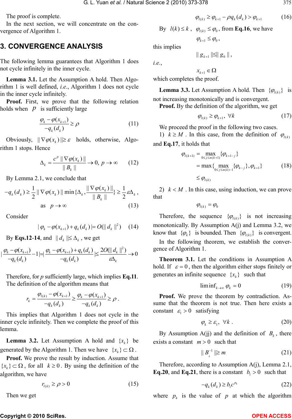



 

G. L. Yuan et al. / Natural Science 2 (2010) 373-378
375
The proof is complete.
In the next section, we will concentrate on the con-
vergence of Algorithm 1.
3. CONVERGENCE ANALYSIS
The following lemma guarantees that Algorithm 1 does
not cycle infinitely in the inner cycle.
Lemma 3.1. Let the Assumption A hold. Then Algo-
rithm 1 is well defined, i.e., Algorithm 1 does not cycle
in the inner cycle infinitely.
Proof. First, we prove that the following relation
holds when
p
is sufficiently large
1
()
()
kk
kk
x
qd




 (11)
Obviously, ||() ||
k
x

  holds, otherwise, Algo-
rithm 1 stops. Hence
||() ||0,
|| ||
p
k
k
k
cx p
B
 
  (12)
By Lemma 2.1, we conclude that
||() || 11
()||()|| min{,}
2||||2
k
kkkkk
k
x
qd xB




  ,
as p (13)
Consider
2
1
|()()|(||||)
kkkk k
xqdOd 

 (14)
By Eqs.12-14, and || ||
kk
d, we get
2
11
()()()2(||||)
|1||| 0
() ()
kk kkkkk
kkkk k
xxqdOd
qd qd
 



 

Therefore, for p sufficiently large, which implies Eq.11.
The definition of the algorithm means that
() 11
() ()
() ()
lk kkk
k
kk kk
xx
rqd qd
 





.
This implies that Algorithm 1 does not cycle in the
inner cycle infinitely. Then we complete the proof of this
lemma.
Lemma 3.2. Let Assumption A hold and {}
k
x
be
generated by the Algorithm 1. Then we have {}
k
x.
Proof. We prove the result by induction. Assume that
{}
k
x, for all 0k. By using the definition of the
algorithm, we have
() 0 lk
r


(15)
Then we get
() 11
()
lkkkkk
qd
 


  (16)
By ()lkk

, ()0lk



, from Eq.16, we have
10k




,
this implies
10
|||| ||||
k
g
g


,
i.e.,
1k
x


which completes the proof.
Lemma 3.3. Let Assumption A hold. Then () {}
lk

is
not increasing monotonically and is convergent.
Proof. By the definition of the algorithm, we get
() 1
,
lk kk



 (17)
We proceed the proof in the following two cases.
1) kM. In this case, from the definition of ()lk

and Eq.17, it holds that
(1) 1
0(1)
max {}
lkk j
jnk



 

1
0()1
max{ max {},}
kj k
jnk



 

(18)
()lk


2) kM

. In this case, using induction, we can prove
that
() 0lk



Therefore, the sequence () {}
lk

is not increasing
monotonically. By Assumption A(j) and Lemma 3.2, we
know that {}
k

is bounded. Then () {}
lk

is convergent.
In the following theorem, we establish the conver-
gence of Algorithm 1.
Theorem 3.1. Let the conditions in Assumption A
hold. If 0


, then the algorithm either stops finitely or
generates an infinite sequence {}
k
x
such that
lim inf0
kk

  (19)
Proof. We prove the theorem by contradiction. As-
sume that the theorem is not true. Then here exists a
constant 10

 satisfying
1, kk

 . (20)
By Assumption A(jj) and the definition of k
B, there
exists a constant 0m such that
1
|| ||
k
Bm
 (21)
Therefore, according to Assumption A(j), Lemma 2.1,
Eq.20, and Eq.21, there is a constant 10b such that
1
() k
p
kk
qd bc (22)
where k
p is the value of p at which the algorithm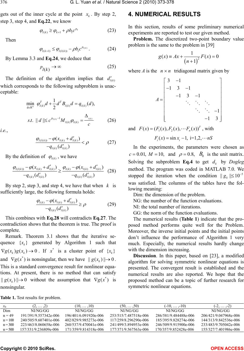

G. L. Yuan et al. / Natural Science 2 (2010) 373-378
376
gets out of the inner cycle at the point k
x
. By step 2,
step 3, step 4, and Eq.22, we know
()1 1
k
p
lk kbc


 (23)
Then
()
(1) (())1
lk
p
lkllk bc

 . (24)
By Lemma 3.3 and Eq.24, we deduce that
()
plk  (25)
The definition of the algorithm implies that ()lk d

which corresponds to the following subproblem is unac-
ceptable:
n()() ()
dR
1
min (),
2
TT
lklklk
ddBdqd 

()
() 1
() ()
.. ||||lk
lk
p
lk lk
st dcMc 


(26)
i.e.,
(())() ()
() ()
()
()
llklk lk
lk lk
xd
qd





  (27)
By the definition of ()lk

, we have
(())() ()()() ()
() ()() ()
() ()
() ()
llklklk lklklk
lk lklk lk
xd xd
qd qd
 
  



(28)
By step 2, step 3, and step 4, we have that when k is
sufficiently large, the following formula holds:
()()()
() ()
()
()
lklk lk
lk lk
xd
qd






 (29)
This combines with Eq.28 will contradicts Eq.27. The
contradiction shows that the theorem is true. The proof is
complete.
Remark. Theorem 3.1 shows that the iterative se-
quence {}
k
x
generated by Algorithm 1 such that
()() 0
kk
gx gx. If *
x
is a cluster point of {}
k
x
and *
()
g
xis nonsingular, then we have ||() ||0
k
gx .
This is a standard convergence result for nonlinear equa-
tions. At present, there is no method that can satisfy
||() ||0
k
gx  without the assumption that * ()
g
x is
nonsingular.
4. NUMERICAL RESULTS
In this section, results of some preliminary numerical
experiments are reported to test our given method.
Problem. The discretized two-point boundary value
problem is the same to the problem in [39]

2
1
()() 0
1
gx AxFx
n



where A is the nn

tridiagonal matrix given by
31
13 1
131
1
13
A




























and 12 ()( (),(),())
T
n
F
xFxFxFx, with
()sin1, i=1,2,
ii
F
xx nS


In the experiments, the parameters were chosen as
0.01,c

10,M

and 0.8,


0
B
is the unit matrix.
Solving the subproblem Eq.4 to get k d by Dogleg
method. The program was coded in MATLAB 7.0. We
stopped the iteration when the condition 5
|||| 10
k
g


was satisfied. The columns of the tables have the fol-
lowing meaning:
Dim: the dimension of the problem.
NG: the number of the function evaluations.
NI: the total number of iterations.
GG: the norm of the function evaluations.
The numerical results (Table 1) indicate that the pro-
posed method performs quite well for the Problem.
Moreover, the inverse initial points and the initial points
don’t influence the performance of Algorithm 1 very
much. Especially, the numerical results hardly change
with the dimension increasing.
Discussion. In this paper, based on [23], a modified
algorithm for solving symmetric nonlinear equations is
presented. The convergent result is established and the
numerical results are also reported. We hope that the
proposed method can be a topic of further research for
symmetric nonlinear equations.
Table 1. Test results for problem.
x0 (2, … ,2) (10, … ,10) (50, … ,50) (-10, … ,-10) (-2, … ,-2)
Dim NI/NG/GG NI/NG/GG NI/NG/GG NI/NG/GG NI/NG/GG
n = 49 191/391/9.557342e-006 196/401/6.091920e-006253/515/7.487518e-006 286/581/9.484488e-006 206/421/9.047968e-006
n = 100 240/505/9.607401e-006 402/829/9.985273e-006117/259/8.296290e-006185/395/9.828274e-006 144/313/9.842536e-006
n = 300 223/463/8.060658e-006 260/537/9.470041e-006241/499/3.894953e-006246/509/9.915900e-006 233/483/9.705042e-006
n = 500 157/331/9.236809e-006 171/359/9.814318e-006177/371/9.567563e-006170/357/9.852428e-006 155/327/7.401986e-006

G. L. Yuan et al. / Natural Science 2 (2010) 373-378
377
REFERENCES
[1] Yuan, G.L. and Lu, X.W. (2009) A modified PRP conju-
gate gradient method. Annals of Operations Research,
166(1), 73-90.
[2] Yuan, G.L. and Lu, X.W. (2008) A new line search
method with trust region for unconstrained optimization.
Communications on Applied Nonlinear Analysis, 15(1),
35-49.
[3] Yuan, G.L. and Wei, Z.X. (2009) New line search meth-
ods for unconstrained optimization. Journal of the Ko-
rean Statistical Society, 38(1), 29-39.
[4] Yuan, G.L. and Wei, Z.X. (2008) Convergence analysis of
a modified BFGS method on convex minimizations.
Computational Optimization and Applications.
[5] Yuan, G.L. and Wei, Z.X. (2008) The superlinear con-
vergence analysis of a nonmonotone BFGS algorithm on
convex objective functions. Acta Mathematica Sinica,
English Series, 24(1), 35-42.
[6] Yuan, G.L. and Lu, X.W. and Wei, Z.X. (2007) New
two-point stepsize gradient methods for solving uncon-
strained optimization problems. Natural Science Journal
of Xiangtan University, 29(1), 13-15.
[7] Yuan, G.L. and Wei, Z.X. (2004) A new BFGS trust re-
gion method. Guangxi Science, 11 , 195-196.
[8] Moré, J.J. and Sorensen, D.C. (1983) Computing a trust-
region step. SIAM Journal on Scientific and Statistical
Computing, 4(3), 553-572.
[9] Flecher, R. (1987) Practical methods of optimization. 2nd
Edition, John and Sons, Chichester.
[10] Gay, D.M. (1981) Computing optimal locally constrained
steps. SIAM Journal on Scientific and Statistical Com-
puting, 2, 186-197.
[11] Powell, M.J.D. (1975) Convergence properties of a class
of minimization algorithms. Mangasarian, O.L., Meyer,
R.R. and Robinson, S.M., Ed., Nonlinear Programming,
Academic Press, New York, 2, 1-27.
[12] Schultz, G.A., Schnabel, R.B. and Bryrd, R.H. (1985) A
family of trust-region-based algorithms for unconstrained
minimization with strong global convergence properties.
SIAM Journal on Numerical Analysis, 22(1), 47-67.
[13] Byrd, R.H., Schnabel, R.B. and Schultz G.A. (1987) A
trust-region algorithm for nonlinearly constrained opti-
mization. SIAM Journal on Numerical Analysis, 24(5),
1152-1170.
[14] Celis, M.R., Dennis, J.E. and Tapia, R.A. (1985) A
trust-region strategy for nonlinear equality constrained
optimization, in numerical optimization 1984. Boggs, P.R.
Byrd, R.H. and Schnabel, R.B., Ed., SIAM, Philadelphia,
71-82.
[15] Liu, X. and Yuan, Y. (1997) A global convergent, locally
superlinearly convergent algorithm for equality con-
strained optimization. Research Report, ICM-97-84,
Chinese Academy of Sciences, Beijing.
[16] Vardi, A. (1985) A trust-region algorithm for equality
constrained minimization: Convergence properties and
implementation. SIAM Journal of Numerical Analysis, 22(3),
575-579.
[17] Nocedal, J. and Yuan, Y. (1998) Combining trust region
and line search techniques. Advances in Nonlinear Pro-
gramming, 153-175.
[18] Sterhaug, T. (1983) The conjugate gradient method and
trust regions in large-scale optimization. SIAM Journal
Numerical Analysis, 20(3), 626-637.
[19] Yuan, Y. (2000) A review of trust region algorithms for
optimization. Proceedings of the 4th International Con-
gress on Industrial & Applied Mathematics (ICIAM 99),
Edinburgh, 271-282.
[20] Yuan, Y. (2000) On the truncated conjugate gradient
method. Mathematical Programming, 87(3), 561-573.
[21] Zhang, X.S., Zhang, J.L. and Liao, L.Z. (2002) An adap-
tive trust region method and its convergence. Science in
China, 45, 620-631.
[22] Yuan, G.L., Meng, S.D. and Wei, Z.X. (2009) A trust-
region-based BFGS method with line search technique
for symmetric nonlinear equations. Advances in Opera-
tions Research, 2009, 1-20.
[23] Zhang, J.L. and Zhang, X.S. (2003) A nonmonotone
adaptive trust region method and its convergence. Com-
puters and Mathematics with Applications, 45(10-11),
1469-1477.
[24] Schnabel, R.B. and Eskow, R. (1990) A new modified
cholesky factorization. SIAM Journal on Scientific and
Statistical Computing, 11(6), 1136-1158.
[25] Griewank, A. (1986) The ‘global’ convergence of Broy-
den-like methods with a suitable line search. Journal of
the Australian Mathematical Society Series B, 28, 75-92.
[26] Zhu, D.T. (2005) Nonmonotone backtracking inexact
quasi-Newton algorithms for solving smooth nonlinear
equations. Applied Mathematics and Computation, 161(3),
875-895.
[27] Fan, J.Y. (2003) A modified Levenberg-Marquardt algo-
rithm for singular system of nonlinear equations. Journal
of Computational Mathematics, 21, 625-636.
[28] Yuan, Y. (1998) Trust region algorithm for nonlinear
equations. Information, 1, 7-21.
[29] Yuan, G.L., Wei, Z.X. and Lu, X.W. (2009) A non-
monotone trust region method for solving symmetric
nonlinear equations. Chinese Quarterly Journal of Mathe-
matics, 24, 574-584.
[30] Yuan, G.L. and Lu, X.W. and Wei, Z.X. (2007) A modi-
fied trust region method with global convergence for
symmetric nonlinear equations. Mathematica Numerica
Sinica, 11(3), 225-234.
[31] Li, D. and Fukushima, M. (1999) A global and superlin-
ear convergent Gauss-Newton-based BFGS method for
symmetric nonlinear equations. SIAM Journal on Nu-
merical Analysis, 37(1), 152-172.
[32] Wei, Z.X., Yuan, G.L. and Lian, Z.G. (2004) An ap-
proximate Gauss-Newton-based BFGS method for solv-
ing symmetric nonlinear equations. Guangxi Sciences,
11(2), 91-99.
[33] Yuan, G.L. and Li, X.R. (2004) An approximate Gauss-
Newton-based BFGS method with descent directions for
solving symmetric nonlinear equations. OR Transactions,
8(4), 10-26.
[34] Yuan, G.L. and Li, X.R. (2010) A rank-one fitting method
for solving symmetric nonlinear equations. Journal of
Applied Functional Analysis, 5(4), 389-407.
[35] Yuan, G.L. and Lu, X.W. and Wei, Z.X. (2009) BFGS
trust-region method for symmetric nonlinear equations.

G. L. Yuan et al. / Natural Science 2 (2010) 373-378
378
Journal of Computational and Applied Mathematics, 230(1),
44-58.
[36] Yuan, G.L., Wei, Z.X. and Lu, X.W. (2006) A modified
Gauss-Newton-based BFGS method for symmetric non-
linear equations. Guangxi Science, 13(4), 288-292.
[37] Yuan, G.L., Wang, Z.X. and Wei, Z.X. (2009) A rank-one
fitting method with descent direction for solving sym-
metric nonlinear equations. International Journal of
Communications, Network and System Sciences, 2(6),
555-561.
[38] Yuan, G.L. and Lu, X.W. (2008) A new backtracking
inexact BFGS method for symmetric nonlinear equations.
Computer and Mathematics with Application, 55(1), 116- 129.
[39] Ortega, J.M. and Rheinboldt, W.C. (1970) Iterative solu-
tion of nonlinear equations in several variables. Aca-
demic Press, New York.