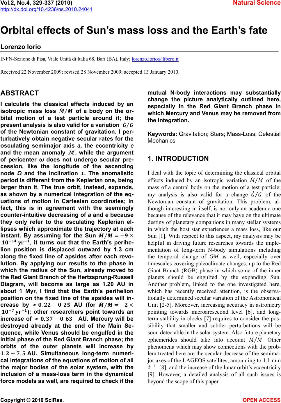
 Vol.2, No.4, 329-337 (2010) Natural Science http://dx.doi.org/10.4236/ns.2010.24041 Copyright © 2010 SciRes. OPEN ACCESS Orbital effects of Sun’s mass loss and the Earth’s fate Lorenzo Iorio INFN-Sezione di Pisa, Viale Unità di Italia 68, Bari (BA), Italy; Ulorenzo.iorio@libero.itU Received 22 November 2009; revised 28 November 2009; accepted 13 January 2010. ABSTRACT I calculate the classical effects induced by an isotropic mass loss of a body on the or- bital motion of a test particle around it; the present analysis is also valid for a variation of the Newtonian constant of gravitation. I per- turbatively obtain negative secular rates for the osculating semimajor axis a, the eccentricity e and the mean anomaly , while the argument of pericenter ω does not undergo secular pre- cession, like the longitude of the ascending node Ω and the inclination I. The anomalistic period is different from the Keplerian one, being larger than it. The true orbit, instead, expands, as shown by a numerical integration of the eq- uations of motion in Cartesian coordinates; in fact, this is in agreement with the seemingly counter-intuitive decreasing of a and e because they only refer to the osculating Keplerian el- lipses which approximate the trajectory at each instant. By assuming for the Sun =× , it turns out that the Earth's perihe- lion position is displaced outward by 1.3 cm along the fixed line of apsides after each revo- lution. By applying our results to the phase in which the radius of the Sun, already moved to the Red Giant Branch of the Hertzsprung-Russell Diagram, will become as large as 1.20 AU in about 1 Myr, I find that the Earth's perihelion position on the fixed line of the apsides will in- crease by .. AU (for =× ); other researchers point towards an increase of .. AU. Mercury will be destroyed already at the end of the Main Se- quence, while Venus should be engulfed in the initial phase of the Red Giant Branch phase; the orbits of the outer planets will increase by .. AU. Simultaneous long-term numeri- cal integrations of the equations of motion of all the major bodies of the solar system, with the inclusion of a mass-loss term in the dynamical force models as well, are required to check if the mutual N-body interactions may substantially change the picture analytically outlined here, especially in the Red Giant Branch phase in which Mercury and Venus may be removed from the integration. Keywords: Gravitation; Stars; Mass-Loss; Celestial Mechanics 1. INTRODUCTION I deal with the topic of determining the classical orbital effects induced by an isotropic variation of the mass of a central body on the motion of a test particle; my analysis is also valid for a change of the Newtonian constant of gravitation. This problem, al- though interesting in itself, is not only an academic one because of the relevance that it may have on the ultimate destiny of planetary companions in many stellar systems in which the host star experiences a mass loss, like our Sun [1]. With respect to this aspect, my analysis may be helpful in driving future researches towards the imple- mentation of long-term N-body simulations including the temporal change of GM as well, especially over timescales covering paleoclimate changes, up to the Red Giant Branch (RGB) phase in which some of the inner planets should be engulfed by the expanding Sun. Another problem, linked to the one investigated here, which has recently received attention, is the observa- tionally determined secular variation of the Astronomical Unit [2-5]. Moreover, increasing accuracy in astrometry pointing towards microarcsecond level [6], and long- term stability in clocks [7] requires to consider the pos- sibility that smaller and subtler perturbations will be soon detectable in the solar system. Also future planetary ephemerides should take into account . Other phenomena which may show connections with the prob- lem treated here are the secular decrease of the semima- jor axes of the LAGEOS satellites, amounting to 1.1 mm d1 [8], and the increase of the lunar orbit’s eccentricity [9]. However, a detailed analysis of all such issues is beyond the scope of this paper.  330 L. Iorio / Natural Science 2 (2010) 329-337 Copyright © 2010 SciRes. OPEN ACCESS Many treatments of the mass loss-driven orbital dy- namics in the framework of the Newtonian mechanics, based on different approaches and laws of variation of the central body’s mass, can be found in literature [2,4,10-18] and references therein. The plan of the paper is as follows. Section 2 is de- voted to a theoretical description of the phenomenon in a two-body scenario. By working in the Newtonian frame- work, I will analytically work out the changes after one orbital revolution experienced by all the Keplerian orbit- al elements of a test particle moving in the gravitational field of a central mass experiencing a variation of its GM linear in time. Then, I will clarify the meaning of the results obtained by performing a numerical integration of the equations of motion in order to visualize the true trajectory followed by the planet. Concerning the me- thod adopted, I will use the Gauss perturbation equations [19,20], which are valid for generic disturbing accelera- tions depending on position, velocity and time, the “standard” Keplerian orbital elements (the Type I acc- ording to [16]) with the eccentric anomaly E as “fast” angular variable. Other approaches and angular variables like, e.g. the Lagrange perturbation equations [19,20], the Type II orbital elements [16] and the mean anomaly could be used, but, in my opinion, at a price of major conceptual and computational difficulties1. With respect to possible connections with realistic situations, it should be noted that, after all, the Type I orbital elements are usually determined or improved in standard data reduc- tion analyses of the motion of planets and (natural and artificial) satellites. Instead, my approach should, hope- fully, appear more transparent and easy to interpret, al- though, at first sight, some counter-intuitive results con- cerning the semimajor axis and the eccentricity will be obtained; moreover, for the chosen time variation of the mass of the primary, no approximations are used in the calculations which are quite straightforward. However, it is important to stress that such allegedly puzzling fea- tures are only seemingly paradoxical because they will turn out to be in agreement with numerical integrations of the equations of motion, as explicitly shown by the Figures depicted. Anyway, the interested reader is ad- vised to look also at [16] for a different approach. In Section 3, I will apply our results to the future Sun-Earth scenario and to the other planets of the solar system. Section 4 summarizes my results. 2. ANALYITICAL CALCULATION OF THE ORBITAL EFFECT OF By defining at a given epoch 0, the accelera- tion of a test particle orbiting a central body experienc- ing a variation of is, to first order in 0, = () 2 21 + (0) , (1) with |=0. will be assumed constant throughout the temporal interval of interest = 0, as it is the case, e.g., for most of the remaining life- time of the Sun as a Main Sequence (MS) star [1]. Note that can, in principle, be due to a variation of both the Newtonian gravitational constant G and the mass M of the central body, so that = + . (2) Moreover, while the orbital angular momentum is conserved, this does not happen for the energy. By limiting ourselves to realistic astronomical scena- rios like our solar system, it is quite realistic to assume that (0)1 (3) over most of its remaining lifetime: indeed, since is of the order of 2 1014 yr 1, for the Sun [1], the con- dition (3) is satisfied for the remaining2 7.58 Gyr before the Sun will approach the RGB tip in the Hertzsprung-Russell Diagram (HRD). Thus, I can treat it perturbatively with the standard methods of celestial mechanics. The unperturbed Keplerian ellipse at epoch 0, as- sumed coinciding with the time of the passage at perihe- lion , is characterized by =(1cos ), =1cos , cos =cos 1cos , sin =12sin 1cos, (4) where a and e are the semimajor axis and the eccentricity, respectively, which fix the size and the shape of the un- changing Keplerian orbit, 3 is its unper- turbed Keplerian mean motion, f is the true anomaly, reckoned from the pericentre, and E is the eccentric anomaly. Eq.4 characterizes the path followed by the particle for any > if the mass loss would sudden- ly cease at . Instead, the true path will be, in general, different from a closed ellipse because of the perturba- tion induced by , and the orbital parameters of the os- culating ellipses approximating the real trajectory at each instant of time will slowly change in time. Think, e.g. , about the cumbersome expansions in terms of the mean anomaly and the Hansen coefficients, the subtleties concerning the choice of the independent variable in the Lagrange equations for the semimajor axis and the eccentricity [19]. About 80% of such a mass- loss is due to the core nuclear burning, while the remaining 20% is due to average solar wind. The age of the present-day MS Sun is 4.58 Gyr, counted from its z -age MS star model [1].  L. Iorio / Natural Science 2 (2010) 329-337 331 Copyright © 2010 SciRes. OPEN ACCESS 2.1. The Semimajor Axis and the Eccentricity The Gauss equation for the variation of the semimajor axis a is [19,20] =2 12sin + , (5) where and are the radial and transverse, i.e. orthogonal to the direction of , components, respec- tively, of the disturbing acceleration, and (12) is the semilatus rectum. In the present case == 2, (6) i.e. there is an entirely radial perturbing acceleration. For <0, i.e. a decrease in the body’s GM, the total gravi- tational attraction felt by the test particle, given by (1), is reduced with respect to the epoch . In order to have the rate of the semimajor axis aver- aged over one (Keplerian) orbital revolution (6) must be inserted into (5), evaluated onto the unperturbed Keple- rian ellipse with (4) and finally integrated over 2 from 0 to 2 because 2 1Kep (see below). Note that, from (4), it can be obtained =sin . (7) As a result, I have 4 = (sin )sin (1cos)2 2 0 (8) =2 1 . Note that if decreases, a gets reduced as well: <0. This may be seemingly bizarre and coun- ter-intuitive, but, as it will be shown later, it is not in contrast with the true orbital motion. The Gauss equation for the variation of the eccentric- ity is [19,20] =12 sin +cos +1 1 (9) For = it reduces to =12 2 , (10 ) so that =(1 + ) ; (11) also the eccentricity gets smaller for <0. As a consequence of the found variations of the oscu- lating semimajor axis and the eccentricity, the osculating orbital angular momentum per unit mass, defined by 2(12), remains constant: indeed, by using (8) and (11), it turns out 2 =(12)2=0. (12) The osculating total energy 2 decreases according to = 22= (1) . (13) Moreover, the osculating Keplerian period Kep 23 , (14) which, by definition, yields the time elapsed between two consecutive perihelion crossings in absence of per- turbation, i.e. it is the time required to describe a fixed osculating Keplerian ellipse, decreases according to Kep = 3 2Kep =6 (1) 32 . (15) As I will show, also such a result is not in contrast with the genuine orbital evolution. 2.2. The Pericenter, the Node and the Inclination The Gauss equation for the variation of the argument of pericentre ω is [19,20] =12 cos+1 + sin cos , (16) where I and Ω are the inclination and the longitude of the ascending node, respectively, which fix the orienta- tion of the osculating ellipse in the inertial space. Since and depend on the normal component of the disturbing acceleration, which is absent in the present case, and =, I have =12 2 (sin )(cos) (1cos)2 2 0= 0. (17) The osculating ellipse does not change its orientation in the orbital plane, which, incidentally, remains fixed in the inertial space because =0 and, thus, = = 0. 2.3. The Mean Anomaly The Gauss equation for the mean anomaly , defined as , [19,20] is = 2 12 +cos . (18 ) It turns out that, since 2 =2 ()3(sin ), (19) then 4Recall that the integration is taken over the unperturbed Keplerian ellipse: that is why a and e are kept out of the integral in (8) and in the following averages.  332 L. Iorio / Natural Science 2 (2010) 329-337 Copyright © 2010 SciRes. OPEN ACCESS =+ 2 ; (20 ) the mean anomaly changes uniformly in time at a slower rate with respect to the unperturbed Keplerian case for <0. 2.4. Numerical Integration of the Equations of Motion and Explanation of the Seeming Contradiction with the Analytical Results At first sight, the results obtained here may be rather confusing: if the gravitational attraction of the Sun re- duces in time because of its mass loss the orbits of the planets should expand (see the trajectory plotted in Fig- ure 1, numerically integrated with MATHEMATICA), while I obtained that the semimajor axis and the eccen- tricity undergo secular decrements. Moreover, I found that the Keplerian period Kep decreases, while one would expect that the orbital period increases. In fact, there is no contradiction, and my analytical results do yield us realistic information on the true evo- lution of the planetary motion. Indeed, a, e and Kep refer to the osculating Keplerian ellipses which, at any instant, approximate the true trajectory; it, instead, is not an ellipse, not being bounded. Let us start at from the osculating pericentre of the Keplerian ellipse corres- ponding to chosen initial conditions: let us use a helio- centric frame with the x axis oriented along the osculat- ing pericentre. After a true revolution, i.e. when the true Figure 1. Black continuous line: true trajectory obtained by numerically integrating with MATHEMATICA the perturbed equations of motion in Cartesian coordinates over 2 yr; the disturbing acceleration (1) has been adopted. The planet starts from the perihelion on the x axis. Just for illustrative purposes, a mass loss rate of the order of 102 yr1 has been adopted for the Sun; for the planet initial conditions corresponding to a = 1 AU, e = 0.8 have been chosen. Red dashed line: unper- turbed Keplerian ellipse at =0=. Blue dash-dotted line: osculating Keplerian ellipse after the first perihelion passage. As can be noted, its semimajor axis and eccentricity are clearly smaller than those of the initial unperturbed ellipse. Note also that after 2 yr the planet has not yet reached the perihelion as it would have done in absence of mass loss, i.e. the true orbital period is longer than the Keplerian one of the osculating red ellipse. radius vector of the planet has swept an angular interval of 2, the planet finds itself again on the x axis, but at a larger distance from the starting point because of the orbit expansion induced by the Sun's mass loss. It is not difficult to understand that the osculating Keplerian el- lipse approximating the trajectory at this perihelion pas- sage is oriented as before because there is no variation of the (osculating) argument of pericentre, but has smaller semimajor axis and eccentricity. And so on, revolution after revolution, until the perturbation theory can be ap- plied, i.e. until 1. In Figure 1 the situ- ation described so far is qualitatively illustrated. Just for illustrative purposes I enhanced the overall effect by assuming 102 yr 1 for the Sun; the initial conditions for the planet correspond to an unperturbed Keplerian ellipse with a = 1 AU, e = 0.8 with the present-day value of the Sun's mass in one of its foci. It is apparent that the initial osculating red dashed ellipse has larger a and e with respect to the second osculating blue dash-dotted ellipse. Note also that the true orbital period, intended as the time elapsed between two con- secutive crossings of the perihelion, is larger than the unperturbed Keplerian one of the initial red dashed os- culating ellipse, which would amount to 1 yr for the Earth: indeed, after 2 yr the planet has not yet reached the perihelion for its second passage. Now, if I compute the radial change () in the osculating radius vector as a function of the eccentric anomaly E I can gain useful insights concerning how much the true path has expanded after two consecutive perihelion passages. From the Keplerian expression of the Sun-planet distance in (4) one gets the radial com- ponent of the orbital perturbation expressed in terms of the eccentric anomaly E ()=(1cos )cos +sin; (21) It agrees with the results obtained in [21]. Since =2 sin cos 1cos, =12 sin cos 1cos , =+sin 1cos =1 [()+()+()], (22) with ()=2+2(cos 1) 1cos, ()=12 1+(1+)cossin (1cos)2 ()=12sin (sincos ) (1cos)2, ( 23) It follows ()= [()+()], (24)  L. Iorio / Natural Science 2 (2010) 329-337 333 Copyright © 2010 SciRes. OPEN ACCESS with ()= 2(sin cos )+ +sin 2+2(cos 1) 1cos 12sin 2(sin cos ) (1cos )2 , (25) and ()= 1 2 1cos cos ( sin cos ) + +sin 1+ ( 1+ ) cos sin 1cos . (26) It turns out from (25) and (26) that, for E > 0, (E) never vanishes; after one orbital revolution, i.e. after that an angular interval of 2 has been swept by the (osclat- ing) radius vector, a net increase of the radial (osculating) distance occurs according to5 (2)(0)=(2)=2 (1) (27) This analytical result is qualitatively confirmed by the difference6 () between the radial distances obtained from the solutions of two numerical integrations of the equations of motion over 3 yr with and without ; the initial conditions are the same. For illustrative purposes I used a = 1 AU, e = 0.01, =0.1 yr1. The result is depicted in Figure 2. Note also that (25) and (26) tell us that the shift at the aphelion is ()=1 21+ 1(2), (28) in agreement with Figure 1 where it is 4.5 times larger than the shift at the perihelion. Since Figure 1 tells us that the orbital period gets larger than the Keplerian one, it means that the true orbit must somehow remain behind with respect to the Keple rian one. Thus, a negative perturbation in the trans- verse direction must occur as well; see Figure 3. Let us now analytically compute it. According to [21], it can be used =sin 12+12+(+cos ). (29) By recalling that, in the present case, = 0 and using =12 1+(1+)cossin 1cos, (30) it is possible to obtain from (22) and (30) (31) with Figure 2. Difference () between the radial distances ob- tained from the solutions of two numerical integrations with MATHEMATICA of the equations of motion over 3 yr with and without ; the initial conditions are the same. Just for illustrative purposes a mass loss rate of the order of = 0.1 yr1 has been adopted for the Sun; for the planet initial conditions corresponding to a = 1 AU, e = 0.01 have been chosen. The cumulative increase of the Sun-planet distance induced by the mass loss is apparent. Figure 3. Radial and transverse perturbations and of the Keplerian radius vector (in blue); the presence of the transverse perturbation makes the real orbit (in red) lag- ging behind the Keplerian one. ()=sin (cossin ), ()= (1cos ) [(1 + )(cos 1)+sin ], ()= 2 + 2(cos 1), ()=sin 1 2 (cossin) 1cos , ()= 1 2 (1+)(1cos )sin 1cos . (32) It turns out from (31) and (32) that, for > 0, () never vanishes; at the time of perihelion passage (2)(0)=42 1+ 1 <0. (33) According to (25) and (26), r(0) = 0. Strictly speaking, r and the quantity plotted in Figure 2 are different objects, but, as the following discussion will clarify, I can assume that, in practice, they are the same.  334 L. Iorio / Natural Science 2 (2010) 329-337 Copyright © 2010 SciRes. OPEN ACCESS This means that when the Keplerian path has reached the perihelion, the perturbed orbit is still behind it. Such features are qualitatively confirmed by Figure 1. From a vectorial point of view, the radial and transverse pertur- bations to the Keplerian radius vector r yield a correc- tion = + , (34 ) so that pert =+. (35) The length of is ()=()2+()2. (36) Eqs.27 and 31 tell us that at perihelion it amounts to (2)=(2)1 + 42(1+) (1)3 . (37) The angle ξ between and r is given by tan () = () (); (38) at perihelion it is tan (2)= 21+ (1)32 , (39) i.e. ξ is close to 90 deg; for the Earth it is 81.1 deg. Thus, the difference between the lengths of the perturbed radius vector pert and the Keplerian one r at a given instant amounts to about cos ; (40) in fact, this is precisely the quantity determined over 3 yr by the numerical integration of Figure 2. At the perihe- lion I have =(2)1 + 42(1 + ) (1)3 cos . (41) Since for the Earth 1 + 42(1+) (1)3 cos =1.0037, (42) it holds (2). (43) This explains why Figure 2 gives us just . Concerning the observationally determined increase of the Astronomical Unit, more recent estimates from processing of huge planetary data sets by Pitjeva point towards a rate of the order of 102 m yr 1 [22,23]. It may be noted that my result for the secular variation of the terrestrial radial position on the line of the apsides would agree with such a figure by either assuming a mass loss by the Sun of just 9 × 10¹⁴ yr1 or a decrease of the Newtonian gravitational constant. . Such a value for the temporal varia- tion of G is in agreement with recent upper limits from Lunar Laser Ranging [24]. . This possibility is envisaged in [25] whose authors use = by speaking about a small radial drift of –(6 ± 13)×102 m yr1 in an orbit at 1 AU. 3. THE EVOLUTION OF THE EARTH-SUN SYSTEM In this Section 1 will not consider other effects which may affect the final evolution of the Sun-Earth system like the tidal interaction between the Earth and the tidal bulges of the giant solar photosphere, and the drag fric- tion in the motion through the low chromosphere [1]. For the Earth, by assuming the values a = 1.00000011 AU, e = 0.01671022 at the epoch J2000 (JD 2451545.0) with respect to the mean ecliptic and equinox of J2000 and =9 × 10¹⁴ yr 1, (24) yields (2)=1.3 × 10²m. (44) This means that at every revolution the position of the Earth is shifted along the true line of the apsides (which coincides with the osculating one because of the absence of perihelion precession) by 1.3 cm. This result is con- firmed by our numerical integrations and the discussion of Section 2; indeed, it can be directly inferred from Figure 2 by multiplying the value of at t = 1 yr by 9 × 1013. By assuming that the Sun will continue to lose mass at the same rate for other 7.58 Gyr, when it will reach the tip of the RGB in the HR diagram [1], the Earth will be only 6.7 × 10⁴ AU more distant than now from the Sun at the perihelion. Note that the value 9 × 10¹⁴ yr 1 is an upper bound on the magnitude of the Sun’s mass loss rate; it might be also smaller [1] like, e.g., 7 × 10¹⁴ yr1 which would yield an increment of 5.5 × 10⁴ AU. Concerning the effect of the other planets during such a long-lasting phase, a detailed cal- culation of their impact is beyond the scope of the present paper. By the way, I wish to note that the depen- dence of (2) on the eccentricity is rather weak; indeed, it turns out that, according to (24), the shift of the perihelion position after one orbit varies in the range 1.1 1.3 cm for 00.1 . Should the interaction with the other planets increase notably the eccentricity, the expansion of the orbit would be even smaller; indeed, for higher values of e like, e.g., e = 0.8 it reduces to about 3 mm. By the way, it seems that the eccentricity of the Earth can get as large as just 0.02 – 0.1 [26-28] over timescales of 5 Gyr due to the N-body interactions with the other planets. In Table 1, I quote the expansion of the orbits of the other planets of the solar system as well.  L. Iorio / Natural Science 2 (2010) 329-337 335 Copyright © 2010 SciRes. OPEN ACCESS It is interesting to note that Mercury7 and likely Venus are fated at the beginning of the RGB; indeed, from Figure 2 of [1] it turns out that the Sun’s photosphere will reach about 0.5-0.6 AU, while the first two planets of the solar system will basically remain at 0.38 AU and 0.72 AU, respectively, being the expansion of their orbits negligible according to Table 1. After entering the RG phase things will dramatically change because in only 1 Myr the Sun will reach the tip of the RGB phase loosing mass at a rate of about 2 × 10⁷ yr1 and expanding up to 1.20 AU [1]. In the meantime, according to our perturbative calculations, the perihelion distance of the Earth will increase by 0.25 AU. I have used as initial conditions for , a and e their final values of the preceding phase 7.58 Gyr-long. In Table 2, I quote the expansion experienced by the other planets as well; it is interesting to note that the outer planets of the solar system will undergo a considerable increase in the size of their orbits, up to 7.5 AU for Neptune, contrary to the conclusions of the numerical computations in [29] who included the mass loss as well. I have used as initial conditions the final ones of the pre- vious MS phase. Such an assumption seems reasonable for the giant planets since their eccentricities should be left substantially unchanged by the mutual N-body inte- ractions during the next 5 Gyr and more [26-28]; con- cerning the Earth, should its eccentricity become as Table 1. Expansion of the orbits, in AU, of the eight planets of the solar system in the next 7.58 Gyr for =9 × 10¹⁴ yr1. I have neglected mutual N-body interactions. Venus Earth Mars Jupiter Saturn Uranus Neptune 7 × 10⁴ 9 × 10⁴ 3 × 10³ 6 × 10³ 2 Table 2. Expansion of the orbits, in AU, of the eight planets of the solar system in the first 1 Myr of the RGB for = 2 × 10⁷ yr1. I have neglected mutual N-body interactions and other phenomena like the effects of tidal bulges and chro- mospheric drag for the inner planets. Venus Earth Mars Jupiter Saturn Uranus 2.5 × 101 3.4 × 101 1.24 2.25 4.57 large as 0.1 due to the N-body perturbations [26-28], after about 1 Myr its radial shift would be smaller amounting to 0.22 AU. Mutual N-body interactions have not been considered. Thus, orbital hardly preventing our planet to escape from engulfment in the expanding solar photosphere. Concerning the result for the Earth, it must be pointed out that it remains substantially unchanged if I repeat the calculation by assuming a circularized orbit during the entire RGB phase. Indeed, it is possible to show that by adopting as initial values of a and the final ones of the previous phase I get that after 1.5 Myr has changed by 0.30 AU. Note that my results are in contrast with those in [1] whose authors obtain more comfortable values for the expansion of the Earth’s orbit, assumed circular and not influenced by tidal and frictional effects, ranging from 1.37 AU (| |=7 × 10¹⁴ yr 1) to 1.50 AU (| |=8 × 10¹⁴ yr 1) and 1.63 AU (| |=9 × 10¹⁴ yr 1). However, it must be noted that such a conclusion relies upon a perturbative treatment of (1) and by assuming that the mass loss rate is constant throughout the RGB until its tip; in fact, dur- ing such a Myr the term ( ) would get as large as 2 × 101. In fact, by inspecting Figure 4 of [1] it ap- pears that in the last Myr of the RGB a moderate varia- tion of occurs giving rise to an acceleration of the order of 1013 yr2. Thus, a further qua- dratic term of the form (0)2 2 (45) should be accounted for in the expansion of (1). A per- turbative treatment yields adequate results for such a phase 1 Myr long since over this time span (45) would amount to 5 × 10². However, there is no need for detailed calculations: indeed, it can be easily noted that the radial shift after one revolution is (2) 4 . (46) After about 1 Myr (46) yields a variation of the order of 109 AU, which is clearly negligible. 4. CONCLUSIONS I started in the framework of the two-body Newtonian dynamics by using a radial perturbing acceleration linear in time and straightforwardly treated it with the standard Gaussian scheme. I found that the osculating semima- jor axis a, the eccentricity e and the mean anomaly secularly decrease while the argument of pericentre ω remains unchanged; also the longitude of the ascending node Ω and the inclination I are not affected. The radial distance from the central body, taken on the fixed line of the apsides, experiences a secular increase . For the Earth, such an effect amounts to about 1.3 cm yr 1. By numerically integrating the equations of motion in Car- 7It might also escape from the solar system or collide with Venus over 3.5 Gyr from now [26-28].  336 L. Iorio / Natural Science 2 (2010) 329-337 Copyright © 2010 SciRes. OPEN ACCESS tesian coordinates I found that the real orbital path ex- pands after every revolution, the line of the apsides does not change and the apsidal period is larger than the un- perturbed Keplerian one. I have also clarified that such results are not in contrast with those analytically ob- tained for the Keplerian orbital elements which, indeed, refer to the osculating ellipses approximating the true trajectory at each instant. I applied our results to the evolution of the Sun-Earth system in the distant future with particular care to the phase in which the Sun, moved to the RGB of the HR, will expand up to 1.20 AU in order to see if the Earth will avoid to be engulfed by the expanded solar photosphere. My answer is negative because, even considering a small acceleration in the process of the solar mass-loss, it turns out that at the end of such a dramatic phase lasting about 1 Myr the perihe- lion distance will have increased by only 0.22- 0.25 AU, contrary to the estimates in [1] whose authors argue an increment of about 0.37-0.63 AU. In the case of a circular orbit, the osculating semimajor axis remains unchanged, as confirmed by a numerical integration of the equations of motion which also shows that the true orbital period increases and is larger than the unper- turbed Keplerian one which remains fixed. Concerning the other planets, while Mercury will be completely en- gulfed already at the end of the MS, Venus might survive; however, it should not escape from its fate in the initial phase of the RGB in which the outer planets will expe- rience increases in the size of their orbits of the order of 1.2- 7.5 AU. As a suggestion to other researchers, it would be very important to complement my analytical two-body calcu- lation by performing simultaneous long-term numerical integrations of the equations of motion of all the major bodies of the solar system by including a mass-loss term in the dynamical force models as well to see if the N-body interactions in presence of such an effect may substantially change the picture outlined here. It would be important especially in the RGB phase in which the inner regions of the solar system should dramatically change. 5. ACKNOWLEDGEMENTS I thank Prof. K.V. Kholshevnikov, St. Petersburg State University for useful comments and references. REFERENCES [1] Schröder, K.P. and Smith, R.C. (2008) Distant future of the Sun and Earth revisited. Monthly Notices of the Royal Astronomy Society, 386(1), 155-163. [2] Krasinsky, G.A. and Brumberg, V.A. (2004) Secular increase of astronomical unit from analysis of the major planet motions, and its interpretation. Celestial Mecha- nics and Dynamical Astronomy, 90(3-4), 267-288. [3] Standish, E.M. (2005) The astronomical unit now. Transits of Venus: New Views of the Solar System and Galaxy. Proceedings of the IAU Colloquium 196, Kurtz, D.W., Ed., Cambridge University Press, Cambridge, 2004, 163-179. [4] Noerdlinger, P.D. (2008) Solar mass loss, the astronomical unit, and the scale of the solar sys- tem. Uhttp://arxiv.org/abs/0801.3807U [5] Klioner, S.A. (2008) Relativistic scaling of astrono- mical quantities and the system of astronomical units. Astronomy and Astrophysics, 478, 951-958. [6] Jin, W., Imants, P. and Perryman, M. (2008) A giant step: From milli- to micro-arcsecond astrometry. Proceedings of the IAU Symposium 248, Cambridge University Press, Cambridge, 2007. [7] Oskay, W.H., Diddams, S.A., Donley, E.A., Fortier, T. M., Heavner, T.P., Hollberg, L., Itano, W.M., Jefferts, S.R., Delaney, M.J., Kim, K., Levi, F., Parker, T.E. and Bergquist, J.C. (2006) Single-atom optical clock with high accuracy. Physical Review Letters, 97(2), 1-4. [8] Rubincam, D.P. (1982) On the secular decrease in the semimajor axis of Lageos’s orbit. Celestial Mechanics and Dynamical Astronomy, 26(4), 361-382. [9] Williams, J.G. and Boggs, D.H. (2008) DE421 lunar orbit, physical librations, and surface coordinates. 16th International Workshop on Laser Ranging, Poznań, 13-17 October 2008. [10] Strömgren, E. (1903) Über die bedeutung kleiner massenänderungen für die newtonsche centralbewe- gung. Astronomische Nachrichten, 163, 129-136. [11] Jeans, J.H. (1924) Cosmogonic problems associated with a secular decrease of mass. Monthly Notices of the Royal Astronomy Society, 85, 2-11. [12] Jeans, J.H. (1961) Astronomy and cosmogony. Dover, New York. [13] Armellini, G. (1935) The variation of the eccentricity in a binary system of decrasing mass. The Observatory, 58, 158-159. [14] Hadjidemetriou, J.D. (1963) Two-body problem with variable mass: A new approach. Icarus, 2, 440-451. [15] Hadjidemetriou, J. D. (1966) Analytic solutions of the two-body problem with variable mass. Icarus, 5, 34-46. [16] Kholshevnikov, K.V. and Fracassini, M. (1968) Le problème des deux corps avec G variable selon l'hypothèse de dirac. Conferenze dell' Osservatorio Astronomico di Milano-Merate, 1(9), 5-50. [17] Deprit, A. (1983) The secular accelerations in Gylden’s problem. Celestial Mechanics and Dynamical Astrono- nomy, 31(1), 1-22. [18] Kevorkian, J. and Cole, J.D. (1966) Multiple scale and singular perturbation methods. Springer, New York and Berlin. [19] Bertotti, B. Farinella, P. and Vokrouhlický, D. (2003) Phyiscs of the solar system. Kluwer, Dordrecht. [20] Roy, A.E. (2005) Orbital motion. 4th Edition, Institute of Physics, Bristol. [21] Casotto, S. (1993) Position and velocity perturbations in the orbital frame in terms of classical element pertu- rbations. Celestial Mechanics and Dynamical Astronomy, 55, 209-221. [22] Pitjeva, E. V. (2005) The astronomical unit now. Transits  L. Iorio / Natural Science 2 (2010) 329-337 337 Copyright © 2010 SciRes. OPEN ACCESS of Venus: New Views of the Solar System and Galaxy. Proceedings of the IAU Colloquium 196, 2004, Kurtz, D. W., Ed., Cambridge University Press, Cambridge, 177. [23] Pitjeva, E.V. (2008) Personal communication to P. Noerdlinger. [24] Müller, J. and Biskupek, L. (2007) Variations of the gravitational constant from lunar laser ranging data. Classical and Quantum Gravity, 24, 4533-4538. [25] Williams, J.G., Turyshev, S. G. and Boggs, D. H. (2007) Williams, Turyshev, and Boggs reply. Physical Review Letters, 98(55). [26] Laskar, J. (1994) Large-scale chaos in the solar system. Astronomy and Astrophysics, 287, L9-L12. [27] Ito, K. and Tanikawa, K. (2002) Long-term integra- tions and stability of planetary orbits in our solar system. Monthly Notices of the Royal Astronomy Society, 336, 483-500. [28] Laskar, J. (2008) Chaotic diffusion in the solar system. Icarus, 196, 1-15. [29] Duncan, M.J. and Lissauer, J.J. (1998) The effects of post-main-sequence solar mass loss on the stability of our planetary system. Icarus, 134, 303-310.
|