Vol.2, No.4, 320-328 (2010) Natural Science
http://dx.doi.org/10.4236/ns.2010.24040
Sufficient noise and turbulence can induce
phytoplankton patchiness
Hiroshi Serizawa1, Takashi Amemiya2, Kiminori Itoh1
1 Graduate School of Engineering, Yokohama National University, Yokohama, Japan;
2 Graduate School of Environment and Information Sciences, Yokohama National University, Yokohama, Japan;
Received 25 November 2009; revised 28 December 2009; accepted 3 February 2010.
ABSTRACT
Phytoplankton patchiness ubiquitously obser-
ved in marine ecosystems is a simple phy- sical
phenomenon. Only two factors are required for
its formation: one is persistent variations of
inhomogeneous distributions in the phytopl-
ankton population and the other is turbulent
stirring by eddies. It is not necessary to assume
continuous oscillations such as limit cycles for
realization of the first factor. Instead, a certain
amount of noise is enough. Random fluctua-
tions by environmental noise and turbulent ad-
vection by eddies seem to be common in open
oceans. Based on these hypotheses, we pro-
pose seemingly the simplest method to simulate
patchiness formation that can create realistic
images. Sufficient noise and turbulence can
induce patchiness formation even though the
system lies on the stable equilibrium conditions.
We tentatively adopt the two-component model
with nutrients and phytoplankton, however, the
choice of the mathematical model is not essen-
tial. The simulation method proposed in this
study can be applied to whatever model with
stable equilibrium states including one-com-
ponent ones.
Keywords: Eddy; Fluctuation; Noise; Patchiness;
Reaction-Advection-Diffusion Model; Turbulence
1. INTRODUCTION
Patchiness is the inhomogeneous distribution of phyto-
plankton observed all over the oceans from the tropic to
the boreal zone (Figure 1). The characteristic pattern
with stretched and curled structures appears in the
mesoscale or sub-mesoscale region from one to hun-
dreds of kilometers, where the surface flow is approxi-
mately two-dimensional, i.e., horizontal [1]. This obser-
vation suggests that the main cause of the phenomenon
is referred to the physical factors such as lateral turbu-
lent stirring and mixing by currents and eddies.
It is well known that the spatially inhomogeneous
patterns can be generated in reaction-diffusion or reac-
tion-advection-diffusion systems with equal diffusivities.
One of the remarkable studies using reaction-diffusion
equations was conducted by Medvinsky et al. [2]. They
demonstrated that the diffusive instability can lead the
system to spatiotemporal chaos even though starting
from simple initial conditions. However, the chaotic
patterns arising from reaction-diffusion systems do not
necessarily mimic the real phytoplankton patchiness as
seen in Figure 1. Without advection terms, stretched and
curled structures characteristic of marine patchiness are
not properly reproduced.
The situation is much improved by incorporating the ef-
fects of advection into the model. The simulation images
created by reaction-advection-diffusion systems seem to
show a closer similarity to real patchiness patterns than
those by reaction-diffusion systems [3-6]. The studies by
reaction-advection-diffusion systems usually adopt the
seeded-eddy model to represent two-dimensional turbulent
flows, which is developed by Dyke and Robertson [7].
However, the controversy is that the above mentioned
studies using reaction-diffusion or reaction-advection-dif-
fusion equations assume the limit cycle oscillations as the
origin of heterogeneity in phytoplankton distributions.
Considering that the system with the stable equilibrium
state is meant to be homogeneous even though the initial
state is heterogeneous [8], any pattern formation seems to
require some kind of mechanisms such as limit cycles that
continue to oscillate the system. However, it is not clear
whether the limit cycle oscillations are usual events in
natural aquatic ecosystems. Limit cycle oscillations could
be too severe for the precondition of patchiness formation.
To avoid the contradiction, it is necessary to seek the alter-
native mechanism other than the limit cycle oscillation.
One of the candidates that can replace the limit cycle
oscillation could be persistent noise, which also can pro-
vide continuous changes of phytoplankton population.

H. Serizawa et al. / Natural Science 2 (2010) 320-328
321
Recently, Vainstein et al. [9] examined the stochastic
population dynamics in the turbulent field, using a
two-component reaction-advection-diffusion model
with phytoplankton and zooplankton. In their model,
the equation of zooplankton only contains the noise
term for the reason that the population of zooplankton
is considerably smaller than that of phytoplankton and
thus subject to stochastic processes. The zooplankton
distribution shows the finer structure than the phyto-
plankton distribution in their simulations, which is
consistent with field observations. However, the phyto-
plankton distribution reproduced by their model does
not seem to resemble real satellite images such as
Figure 1.
Ecological systems are open systems in which the
interactions with the external environment are noisy
[10,11]. Thus, it is natural to incorporate random
fluctuations into the model. However, proper incor-
poration of noise is not easy. For example, there are
mathematically two types of noise: one is the additive
noise and the other is the multiplicative noise [12].
The multiplicative noise is dependent on the dynami-
cal variables, while the additive noise is independent
of them. The multiplicative noise is thought to be
caused by the interaction between the corresponding
component and the external environment [10,13].
However, clear criteria do not necessarily exist for
which type of noise should be used in a given situa-
tion. The decision rests more or less on the individual
modeler.
The technical problem in computer simulations is
more crucial. The stochastic spatiotemporal simula-
tions of the partial differential equation model are
strongly affected by such factors as the spatial corre-
lation length and the temporal frequency of random
noise. Therefore, it is important to determine appro-
priate values for these parameters in order that the
effects of noise are properly reflected to simulation
processes. In particular, the temporal frequency of
noise is subtle to be handled. If the changing speed of
noise is too fast or the period of subsequent noise is
too short, successful pattern formation cannot be ex-
pected.
The goal of this paper is to specify the ultimate
causes for patchiness formation and to propose a sim-
ple and convenient simulation method for its repro-
duction. We construct the model on the basis of the
same concept as that by Vainstein et al. [9]. That is,
the model includes the effect of temporally fluctuating
noise as well as those of diffusion and advection.
However, the substantial difference lies on the way to
incorporate noise into the model. The simulation im-
ages obtained by our method seem to show a striking
resemblance to real patchiness patterns as seen in
Figure 1.
Figure 1. Algal blooms in the Barents Sea (Credit: NASA
Goddard Space Flight Center).
Our two-component model consists of nutrients and
phytoplankton. However, the model itself is not essential.
The simulation method used in this study is not only
effective for a wide range of parameter settings but also
applicable to other mathematical models. Robustness
and applicability could afford considerable credibility to
our method.
2. MATHEMATICAL MODEL
2.1. Mean-Field Model
First, we present the mean-field model that describes the
biological interaction. The ordinary differential equa-
tions are given as follows:
,NmP
NH
N
kI
dt
dN
N
N
N

  (1)
.Pm
PH
P
fP
NH
N
I
dt
dP
P
P
P
N
P



  (2)
Two state variables N and P represent the nutrient
concentration (the unit is mmol/m3) and the phytoplank-
ton density (the unit is g/m3), respectively. The other
variable t is actual time (the unit is day). With regard to
the parameters, IN and IP are the input rates of nutrients
and phytoplankton from the external environment, μ is
the maximum growth rate of phytoplankton, k is the nu-
trient content in phytoplankton, fP is the maximum pre-
dation rate of zooplankton on phytoplankton, mN is the
removal rate of nutrients from the system, mP is the
natural mortality rate of phytoplankton, and HN and HP
are the half-saturation constants of nutrients and phyto-

H. Serizawa et al. / Natural Science 2 (2010) 320-328
322
Table 1. Parameters in minimal NP models Eqs.1 and 2 and Eqs.7-9.
Parameters Meanings Set I Set II Units
IN Input rate of nutrients 0.4 0.15 mmol･m-3･day-1
k Nutrient content in phytoplankton 0.2 0.2 mmol/g
HN Half-saturation constant of nutrients 0.2 0.2 mmol/m3
mN Removal rate of nutrients 0.1 0.02 day-1
IP Input rate of phytoplankton 0.04 0.04 g･m-3･day-1
μ Maximum growth rate of phytoplankton 0.5 0.5 day-1
fP Maximum feeding rate of zooplankton on phytoplankton 2.0 2.0 g･m-3･day-1
HP Half-saturation constant of phytoplankton 4.0 4.0 g/m3
mP Mortality rate of phytoplankton 0.1 0.1 day-1
D Diffusion coefficient 0.125 0.125 km2/day
rc Radius of eddies 10.0 (20.0) 10.0 km
Vmax Maximum velocity 10.0 (10.0) 10.0 km/day
Vav Average velocity 2.98 (3.50) 2.98 km/day
L Half length of square domain side 100 100 km
The Set I is used for the simulations in Figures 5, 6 and 7, while the Set II is used in Figure 8. The values within parentheses in the Set I correspond
to the VF I in Figure 2(a), which is used only for the simulation in Figure 6(a).
plankton, respectively. The mathematical model Eqs.1 and
2, named the minimal NP model in the present study, is
known to show both bistability and limit cycle oscillations
for the parameter values within the realistic range [6,8]. The
meanings and the units of these parameters are listed in
Table 1 together with their values.
It is worth pointing out that the input term of phyto-
plankton IP and the removal term of nutrients mNN contrib-
ute to stabilizing the system. For example, the situation that
the phytoplankton density P = 0, where phytoplankton con-
tinue to be extinct, can be avoided by the parameter IP.
Moreover, even if P = 0, the other unfavorable situation that
the nutrient concentration N continues to increase unlimit-
edly can be avoided by the term mNN.
2.2. Velocity Field
Turbulent stirring is considered to be a crucial factor in
creating phytoplankton patchiness in marine ecosystems.
In this study, we use a simplified version of the seeded-
eddy model as two-dimensional turbulent flows [3,6,7,9,
14]. The stream function ψ and fluid velocity V are de-
scribed as follows:
.,),(,1or1
,
2
)()(
exp),( 2
22
2























 
xy
VV
r
yyxx
rAyx
yxi
ii
ii
ii



V
(3)
Suppose that the number of eddies is denoted by n.
Then, the velocity field is composed of n eddies, the half
of which rotate clockwise, while the other half rotate
counter-clockwise. The center of each eddy (xi, yi) is
randomly dispersed within the domain. For simplicity,
we use a constant value of the radius ri for all eddies
without considering a distribution of variant eddy sizes.
Thus, ri = rc (constant). It is supposed that the velocity
field is mainly composed by eddies with larger radii,
because the stream function ψ is proportional to the
square of the radius ri
2. The use of the constant radius
can be justified for this reason. In fact, no essential dif-
ference is observed in the final appearance of patchiness
patterns as compared to the case in which the eddy sizes
are varied. The adoption of the constant radius is for
the sake of speedy simulations. The scaling constant A
is introduced for the adjustment of the maximum ve-
locity Vmax.
Figure 2 shows the velocity fields V used in the
present study. The number and the radius of eddies are
n = 40 and rc = 20 km in Figure 2(a), while n = 100 and
rc = 10 km in Figure 2(b). The former velocity field is
referred to as the VF I, and the latter is as the VF II. In
most of the simulations except for Figure 6(a), the VF II
is employed. The domain is a 200 km × 200 km square,
that is, a half length of each side is L = 100 km. The
maximum velocity Vmax is set up at 10 km/day for both
velocity fields by varying the scaling parameter A. Then,

H. Serizawa et al. / Natural Science 2 (2010) 320-328
323
the average velocities become 3.50 km/day in the VF I,
while 2.98 km/day in the VF II. Both velocity fields are
stationary and remain temporally unchanged, and also
meet the periodic boundary conditions.
2.3. White Noise Process
Random fluctuations are constructed as explained in our
previous study [8]. First, we provide a fluctuation func-
tion to describe a spatially smoothed deviation. The
fluctuation function is formulated using the following
Gaussian distribution function:










2
22
,2
)()(
exp),( s
yyxx
yxGii
i
yxi (4)
The function G depicts a convex curved surface
whose peak locates at (xi, yi), and the peak value equals 1.
Here, the parameter s denotes the correlation length of
fluctuations. The convex Gaussian function G is named the
plus-type, and we can also formulate the minus-type
Gaussian function, denoted as -G, that creates a con-
cave valley.
Thereafter, a total of 100 Gaussian functions are pro-
vided with different (xi, yi) values, which consist of 50
plus-type ones and 50 minus-type ones. As the location
of the peak or the valley (xi, yi) is randomly dispersed
within the domain, the unevenly waved surface can be
generated by the superposition of these Gaussian func-
tions, the average height of which equals 0. Then, the
fluctuation function F is defined as follows:
.1or1,),(),( , i
i
i
yxi yxGyxF i
 (5)
The position coordinates of peaks and valleys (xi, yi)
are different depending on the index i.
Assuming that the peak position (xi, yi) is a function of
time t, the fluctuation function F is also a function of t,
thus, F(x, y, t). Then, we can use the function F(x, y, t) as
time-dependent fluctuations δN,P(x, y, t) for both the nu-
trient concentration N and the phytoplankton density P
according to the following equation:
).,,(),,( ,, tyxFAtyx PNPN

(6)
Here, the parameter AN and AP denote the scale factors
of fluctuations for nutrients and phytoplankton. The
functions δN,P(x, y, t) are referred to as the noise distribu-
tion function in this study. For example, the noise distri-
butions for phytoplankton by δP(x, y, t) are shown in
Figure 3 for three elapsed time, where Figure 3(a) is the
initial distribution of δP(x, y, t) when t = 0. The noise
distribution function δP(x, y, t) continues to change alike,
thereafter, and δN(x, y, t) changes as well.
2.4. Reaction-Advection-Diffusion Model
Finally, we construct the reaction-advection-diffusion
model that synthesizes the above-mentioned factors, that
Figure 2. Velocity fields by turbulent stirring. The velocity field is
constructed by the superimposition of n eddies with the constant
radius rc. (a) n = 40, rc = 20 km. (b) n = 100, rc =10 km. These are
named the VF I and the VF II, respectively. The velocity fields
meet the periodic boundary conditions.
is, the biological interaction, turbulence and noise. Using
the right side of the Eqs.1 an d 2, we can formulate the
following two-dimensional reaction-advection-diffu-
sion model:
),,,(
)(
2
tyxNNm
P
NH
N
kINND
t
N
NN
N
N




V
(7)
).,,(
)(
2
tyxPPm
PH
P
f
P
NH
N
IPPD
t
P
PP
P
P
N
P








V
(8)
The Laplacian operators are described as follows:
.,, 2
2
2
2
2
yx
yx 

















 (9)
The variables x and y are the horizontal position coor-
dinates (the unit is km). The parameter D denotes the
lateral diffusivity, which is equal for two components.
Further, the vector V represents the velocity field shown
in Figure 2. It should be noted that the units of state
variables N and P are changed to mmol/m2 and g/m2 due
to the adoption of the two-dimensional model.
As stated previously, there are two types of noise, the
additive noise and the multiplicative noise. The mathe-
matical model Eqs.7-9 contains the stochastic fluctua-
tion terms in the right-hand sides of the partial differen-
tial equations, which are described in the multiplicative
forms as +NδN(x, y, t) for nutrients and +PδP(x, y, t) for
phytoplankton. This is because we assume the interac-
tions with the external environment for both nutrients
and phytoplankton. However, even if the additive noise
is added for both components, the results are hardly af-
fected. Thus, which type of noise is used is not essential
in the current study. What is important is to set the am-
plitude of noise within adequate values by adjusting the
scale parameters AN and AP in order to avoid the situation

H. Serizawa et al. / Natural Science 2 (2010) 320-328
324
Figure 3. Spatiotemporal variation of noise distribution for phytoplankton. The distribution of noise for the
phytoplankton density P is represented by the noise distribution function δP(x, y, t). (a) shows the initial distri-
bution δP(x, y, 0), which is changed to (b) and (c) consecutively. The noise distributions also meet the periodic
boundary conditions.
Figure 4. White noise processes at (0, 0). These line graphs show the temporal change of the noise dis-
tribution function δP(x, y, t) for phytoplankton at the center of the domain, i.e., δP(0, 0, t). The time step of
the simulations Δt = 0.1 day, meaning that the calculation is carried out 10 times a unit time, which equals
a day. Renewed noise distribution functions are provided every time step in (a) and every 10 time steps,
i.e., everyday in (b), respectively. Also in (b), the amplitude of noise is changed linearly at each time step
between two days. The white noise processes described in (a) and (b) are named the WN I and the WN II,
respectively.
that the population of the component falls to the negative
values.
In white noise processes, the amplitude of the fluctua-
tion, i.e., deviation from the mean value is randomly
distributed within a certain range at each cell and each
unit time. If the difference of the amplitude between
adjacent cells or subsequent time steps is too large, the
system is often led to divergence.
The temporal change of fluctuations is determined as
follows. According to the noise distribution functions
δN,P(x, y, t), the amplitudes of fluctuations for both nu-
trients and phytoplankton change independently at
each cell. Assuming that the time step of the simulation
Δt = 0.1 day, the calculations are conducted ten times a
unit time, i.e., a day. Further, the noise distribution func-
tions δN,P(x, y, t) are renewed every time step (Figure
4(a)) or every ten time steps (Figure 4(b)). In the latter
case, the renewal of δN,P(x, y, t) is performed every unit
time, i.e., everyday, and the amplitude of fluctuations
varies linearly between successive two distributions. The
temporal change of random noise for the phytoplankton
density P at the center of the domain δP(0, 0, t) is de-
picted in Figure 4 for these two cases, which are re-
ferred to as the WN I and the WN II, respectively. The
WN I is used only for the simulation in Figure 7(a).
Otherwise, the WN II is employed.
In our spatiotemporal simulations, the domain is a
200 km × 200 km square, and a half length of each side
L = 100 km. Then, the two-dimensional square domain is
divided into a rectangular grid of 200 × 200 cells. There-
fore, each cell is a 1.0 km × 1.0 km square, and the noise
distribution functions δN,P(x, y, t) are allocated to each
cell. In the initial state, the distribution of both compo-
nents are homogeneous, however, inhomogeneous dis-
tributions are realized just after the onset of simulations
due to random fluctuations. The fourth order Runge-
Kutta integrating method is applied with a time step Δt = 0.1
day, and the periodic boundary conditions are imposed.

H. Serizawa et al. / Natural Science 2 (2010) 320-328
325
It is confirmed that the results with smaller time steps
remain the same for each program, ensuring the accu-
racy of the simulations.
3. RESULTS
3.1. Simulations with Noise (Set I)
Prior to spatiotemporal simulations of the reaction-advec-
tion-diffusion model Eqs.7-9, we conduct the stability
analyses of the mean-field model Eqs.1 and 2. The results
are shown in Table 2. For the parameter Set I in Table 1,
the systems Eqs.1 and 2 have only one fixed point. As the
real parts of two eigenvalues are both negative, this fixed
point is identified as an attractor that represents the stable
equilibrium state. Therefore, even if the initial state is het-
erogeneous, the system is damped out to the uniform distri-
bution in the course of time without continuous fluctuations.
Figure 5 shows the spatiotemporal variation of phyto-
plankton density P for the parameter Set I, in which the
effects of turbulence and noise are both considered. The VF
II given by Figure 2(b) and the WN II described in Figure
4(b) are applied for the simulations. While the initial state is
homogeneous, the spatial distribution of phytoplankton
begins to be disturbed soon due to the combined effects of
furious turbulence and random noise. Then, as early as the
ninth day, patchiness formation is perfectly completed, and
continues to change, thereafter. It should be noted that the
same pattern does not occur again, because the stochastic
perturbation is not periodic.
Table 2. Stability analyses in minimal NP model Eqs.1 and 2.
Set I Set II
(N0, P0) (0.259, 6.631) (1.656, 1.31)
Eigenvalues -0.309 ± 0.029i 0.017 ± 0.037i
Stability Stable Unstable
State Convergence Limit cycle
The minimal NP model Eqs.1 an d 2 generates only one fixed point
(N0, P
0) for both Sets I and II within the region N0 > 0 and P0 > 0,
showing the convergence for the Set I and the limit cycle oscillation
for the Set II, respectively.
The dependence of the patchiness pattern on the tur-
bulence fields are examined in Figure 6. The velocity
fields used in Figure 6(a) and (b) are the VF I and the
VF II in Figure 2, respectively. The broadly extended
structures observed in Figure 6(a) are probably due to
the mildness of currents in the VF I. In contrast, the
stormy velocity field such as the VF II seems to generate
the patchiness pattern with fine structures as seen in
Figure 6(b), showing a clear resemblance with real sat-
ellite images such as Figure 1.
Meanwhile, the dependence on the noise processes is
investigated in Figure 7. The white noise processes cor-
responding to Figures 7(a) and 7(b) are the WN I and
the WN II in Figure 4, respectively. Too frequent change
in the noise distributions could obscure the patchiness
pattern as seen in Figure 7(a). On the contrary, the
patchiness image in Figure 7(b) shows a clear difference
in phytoplankton density. Slowly changing fluctuations
Figure 5. Spatiotemporal variation of phytoplankton distribution in minimal NP model Eqs.7-9. Without noise, the system shows a
convergence to a stable equilibrium state for the parameter Set I in Table 1. However, incorporating random fluctuations into the
model, patchiness formation is induced by the combined effects of turbulence and noise. The VF II and the WN II are employed.
(a) t = 0 day, (b) t = 3 day, (c) t = 6 day, (d) t = 9 day, (e) t = 12 day, (f) t = 15 day.

H. Serizawa et al. / Natural Science 2 (2010) 320-328
326
Figure 6. Dependence of phytoplankton distribution on veloc-
ity field in minimal NP model Eqs.7-9. The parameters are
given by the Set I, and the WN II is employed. t = 15 day.
(a) VF I, (b) VF II (same as Figure 5(f)).
intensify the effects of random noise, facilitating the
emergence of both the densely populated and the spars-
ely populated areas.
3.2. Simulations with Limit Cycle Oscillation
(Set II)
For the comparison, we also survey the pattern forma-
tion in the oscillatory regime. According to the stability
analysis for the parameter Set II, the fixed point of the
system becomes unstable as shown in Table 2, and the
limit cycle is formed around it. In this case, random
noise is not necessary, because the continuous oscillation
encourages the pattern formation unless the initial dis-
tribution is homogeneous [6].
The spatiotemporal variation of phytoplankton density
P for the parameter Set II is shown in Figure 8. Only the
effect of turbulence is considered employing the VF II.
Instead, the initial distributions of both components are
not homogeneous but randomly dispersed. Patchiness
patterns are formed also in this case for the almost same
period as in Figure 5. However, it could be happened
that the similar patterns appear repeatedly with the pe-
riod of the limit cycle oscillation, which was the case in
our previous study [6].
4. DISCUSSIONS
4.1. Comparison with Field Observations
Our simulation results seem to show a close similarity
with satellite images such as Figure 1. Stretched and
curled patterns characteristic of marine patchiness are
clearly reproduced particularly in Figure 5, which em-
ploys energetic turbulence as the VF II and slowly
changing white noise process as the WN II.
We attempt some kinds of numerical comparisons.
First, the size of our simulation images are comparable
to that of the satellite images in Figure 1, which covers
the area of some hundreds kilometers. Considering that
Figure 7. Dependence of phytoplankton distribution on white
noise process in minimal NP model Eqs.7-9. The parameters
are given by the Set I, and the VF II is employed. t = 15 day.
(a) WN I, (b) WN II (same as Figure 5(f)).
most of the patchiness images supplied by NASA are of
a similar size with Figure 1, we can insist that the veloc-
ity field and the noise process adopted in our method are
suitable for patchiness simulations.
Comparing the horizontal diffusivity to experimental
data, two types of diffusion must be distinguished [6,14].
The first type of diffusion is usual diffusion originating
from a tendency toward homogeneity. This type of dif-
fusion is represented by the second order differential for
position coordinates. Thus, the diffusion coefficient D
used in the minimal NP model Eq.7-Eq.9 corresponds to
this type. However, this type of diffusion does not stand
for real diffusion in marine ecosystems. In the context
of computer simulations, diffusion of this type merely
functions as a smoothing factor that prevents divergence
of the system.
Meanwhile, there exists another type of diffusion origi-
nating from advection by currents and eddies, which is
represented by the first order differential for position
coordinates. It is this type of diffusion that is responsible
for patchiness formation in oceanic environments. Thus,
the real diffusion coefficient must be recalculated from
the velocity fields V in Figure 2.
The real diffusion coefficient Dad can be evaluated by
the following equation:
.
2
Dad LD
  (10)
As a rough approximation, suppose that the character-
istic scale of diffusion LD is given by the average veloc-
ity Vav. In the case the VF II in Figure 2(b) is LD ~3.0
km. Then, we can estimate the value of turbulent diffu-
sivity Dad as about 4.5 km2/day. This value is converted
to about 5 × 105 cm2/sec, which is in agreement with the
empirical data estimated by Okubo [15] that range from
5 × 102 to 2 × 106 cm2/sec.
4.2. Crucial Factors for Patchiness Formation
Turbulence and persistent variation of phytoplankton
population are two essential factors for creating marine
patchiness. Particularly as for turbulence, many re-

H. Serizawa et al. / Natural Science 2 (2010) 320-328
327
searchers take it for granted that lateral advection and
mixing by currents and eddies plays a constructive role
for patchiness formation [1]. However, there seems to be
no consensus for another factor at the present time. Ac-
cording to our simulations, both random noise and limit
cycle oscillations can cause persistent variation, and
promote patchiness formation as shown in Figures 5 and
8. It is not yet clear about which is the ultimate cause for
persistent variation of phytoplankton population. Which
is more probable as a crucial factor in patchiness forma-
tion, noise or limit cycles? It seems difficult to judge
from the appearance of simulation images.
Becks et al. [16] reported that a defined chemostat
system with bacteria and ciliate showed dynamic behav-
iors such as chaos and stable limit cycles. In their two-
prey, one-predator system, the changes of the bifurcation
parameter (the dilution rate) trigger the population dy-
namics such as stable coexistence at high dilution rates,
chaos at intermediate dilution rates and stable limit cy-
cles at low dilution rates.
However, there is still a lack of field evidence that
limit cycle oscillations or chaotic behaviors surely occur
in the natural seas and oceans. It seems unnatural to
adopt limit cycle oscillations as a precondition of popu-
lation variations. Thus, it is reasonable to conclude as
follows. That is, random noise ubiquitously observed in
the natural world is the source of persistent variations of
inhomogeneous phytoplankton distributions, which plays a
crucial role in patchiness formation together with turbu-
lent stirring and mixing.
It is worth noting that random noise and limit cycles
are not exclusive. A possibility cannot be denied that
these two contribute together to patchiness formation.
Indeed, further simulations show that the system con-
taining both the noise process and the limit cycle oscilla-
tion can successfully produce realistic patchiness pat-
terns. However, we can insist that the crucial factor is
not limited cycles but noise processes that are responsi-
ble for phytoplankton patchiness in marine ecosystems.
From the technical point of view in computer simula-
tions, appropriate incorporation of turbulence and noise
into the model is indispensable. The effects of these fac-
tors must be fully reflected in the simulations. The ve-
locity field should be sufficiently energetic as the VF II
(Figure 2(b)) rather than the VF I (Figure 2(a)). The
white noise process should be slow enough as the WN II
(Figure 4(b)) rather than the WN I (Figure 4(a)).
4.3. Extension to One-Component Model
In order to confirm robustness and applicability of the
method, we finally attempt the simulation of patchiness
formation using the different model. The exemplified
mathematical model is a partial differential equation
system with one variable, which is described as follows:
).,,(
1)(
2
tyxPPm
PH
P
f
K
P
PIPPD
t
P
PP
P
P
P












V
(11)
The reaction-advection-diffusion model Eq.11 con-
tains only one state variable P, which represents the
phytoplankton density (the unit is g/m2). The parameter
K is the carrying capacity of the environment, and the
meanings of the other parameters are the same as in the
minimal NP models Eqs.1 and 2 and Eqs.7-9. Moreover,
the same velocity field (the VF II) and the same multi-
plicative white noise process (the WN II) as in Figure 5
are employed in the simulation. It should be noted that
limit cycles are impossible due to the use of the one-
variable model. The system can give rise to only a con-
vergence to the attractor, unless it diverges.
Figure 9 is an example of patchiness formation in the
mathematical model Eq.11. The similar pattern forma-
tion with that in Figure 5 proceeds, ensuring robustness
and extensive applicability of the method described in
this study.
5. CONCLUSIONS
1) Phytoplankton patchiness in marine ecosystems is
essentially the physical phenomenon independent of
Figure 8. Spatiotemporal variation of phytoplankton distribution in minimal NP model Eqs.7-9. Without noise, the system shows a
limit cycle oscillation for the parameter Set II in Table 1. In this case, patchiness formation is induced without fluctuations, supposing
that the initial distribution is inhomogeneous. The VF II is employed. (a) t = 0 day, (b) t = 6 day, (c) t = 12 day.

H. Serizawa et al. / Natural Science 2 (2010) 320-328
328
Figure 9. Spatiotemporal variation of phytoplankton distribution in mathematical model Eq.11. Without noise, the sys-
tem shows a convergence to a stable equilibrium state for the following parameters: IP = 0.1 g･m-2･day-1, μ = 0.5 day-1,
K = 20.0 g/m2, fP = 1.6 g･m-2･day-1, HP = 2.4 g/m2, mP = 0.1 day-1. The units are altered to those of the two-dimensional
model. The VF II and the WN II are employed. (a) t = 0 day, (b) t = 6 day, (c) t = 12 day.
each biological process. Turbulence and noise are two
major factors that promote patchiness formation in oce-
anic environments. The pattern formation is guaranteed
by persistent variations of the phytoplankton population.
Stochastic noise is one of the most probable causes re-
sponsible for continuous variations. In addition, stirring
and mixing by currents and eddies facilitate the creation
of stretched and curled structures characteristic of
phytoplankton patchiness.
2) Patchiness formation can be simulated in the spa-
tially extended reaction-advection-diffusion system that
properly integrates the turbulence field and the noise
process. Sufficiently furious turbulence such as the VF II
(Figure 2(b)) and slowly changing fluctuations such as
the WN II (Figure 4(b)) are the key to reproduce realis-
tic images of patchiness.
3) The simulations of patchiness formation can be
performed by whatever model with the stable equilib-
rium state. Robustness in model simulations and appli-
cability to various models could explain the universality
of the phenomenon that is observed worldwide on Earth.
6. ACKNOWLEDGEMENTS
This study is supported by the Global COE Program “Global Eco-Risk
Management from Asian View Points” by the Ministry of Education,
Culture, Sports, Science and Technology, Japan.
REFERENCES
[1] Martin, A.P. (2003) Phytoplankton patchiness: The role
of lateral stirring and mixing. Progress in Oceanography,
57(2), 125-174.
[2] Medvinsky, A.B., Petrovskii, S.V., Tikhonova, I.A.,
Malchow, H. and Li, B.-L. (2002) Spatiotemporal com-
plexity of plankton and fish dynamics. SIAM Review,
44(3), 311-370.
[3] Abraham, E.R. (1998) The generation of plankton patchi-
ness by turbulent stirring. Nature, 391(6667), 577-580.
[4] Neufeld, Z., Haynes, P.H., Garçon, V. and Sudre, J. (2002)
Ocean fertilization experiments may initiate a large scale
phytoplankton bloom. Geophysical Research Letters,
29(11), 1-4.
[5] Tzella, A. and Haynes, P.H. (2007) Small-scale spatial
structure in plankton distributions. Biogeosciences, 4(2),
173-179.
[6] Serizawa, H., Amemiya, T. and Itoh, K. (2008) Patchi-
ness in a minimal nutrient-phytoplankton model. Journal
of Biosciences, 33(3 ), 391-403.
[7] Dyke, P.P.G. and Robertson, T. (1985) The simulation of
offshore turbulent dispersion using seeded eddies. Ap-
plied Mathematical Modelling, 9(6), 429-433.
[8] Serizawa, H., Amemiya, T. and Itoh, K. (2009) Noise-
triggered regime shifts in a simple aquatic model. Eco-
logical Complexity, 6(3), 375-382.
[9] Vainstein, M.H., Rubí, J.M. and Vilar, J.M.G. (2007)
Stochastic population dynamics in turbulent fields. The
European Physical Journal-Special Topics, 146(1), 177-
187.
[10] Spagnolo, B., Valenti, D. and Fiasconaro, A. (2004) Noise in
ecosystems: A short review. Mathematical Biosciences
and Engineering, 1(1), 185-211.
[11] Provata, A., Sokolov, I.M. and Spagnolo, B. (2008) Edi-
torial: Ecological complex systems. The European Physical
Journal B, 65(3), 307-314.
[12] Guttal, V. and Jayaprakash, C. (2007) Impact of noise on
bistable ecological systems. Ecological Modelling, 201
(3-4), 420-428.
[13] Spagnolo, B., Fiasconaro, A. and Valenti, D. (2003)
Noise induced phenomena in Lotka-Volterra systems.
Fluctuation and Noise Letters, 3(2), 177-185.
[14] Serizawa, H., Amemiya, T. and Itoh, K. (2009) Patchi-
ness and bistability in the comprehensive cyanobacterial
model (CCM). Ecological Modelling, 220(6), 764-773.
[15] Okubo, A. (1971) Oceanic diffusion diagram. Deep Sea
Research and Oceanographic Abstracts, 18(8), 789-802.
[16] Becks, L., Hilker, F.M., Malchow, H., Jürgens, K. and
Arndt, H. (2005) Experimental demonstration of chaos in
a microbial food web. Nature, 435(30), 1226-1229.
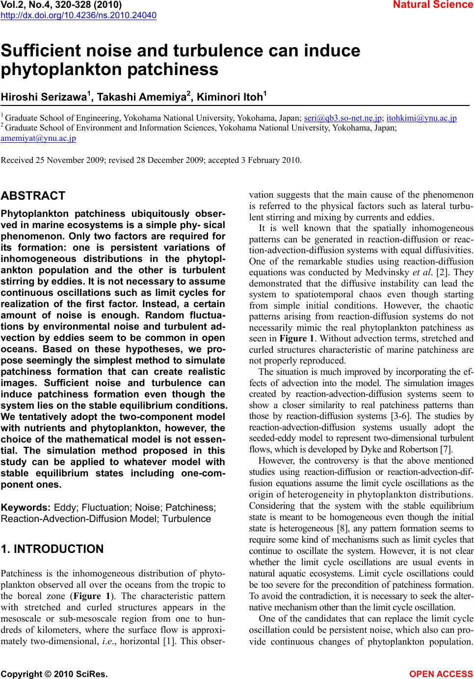