 Modern Instrumentation, 2012, 1, 1-7 http://dx.doi.org/10.4236/mi.2012.11001 Published Online January 2012 (http://www.SciRP.org/journal/mi) A Hybrid Angular/Energy Dispersive Method to Improve Some Characteristics of Laboratory X-Ray Diffraction Valerio Rossi Albertini1, Daniele Bailo1,2, Amanda Generosi1*, Barbara Paci1 1Istituto di Struttura della Materia del CNR, Roma, Italy 2Istituto Nazionale di Geofisica e Vulcanologia, Via di Vigna Murata, Roma, Italy Email: *amanda.generosi@ism.cnr.it Received December 30, 2011; revised January 20, 2012; accepted January 30, 2012 ABSTRACT The Energy Dispersive X-ray Diffraction, generally referred as EDXD, has shown to be a valid alternative to the con- ventional Angular Dispersive X-ray Diffraction, the ADXD. EDXD exhibits several advantages to its AD counterpart, mainly related to the properties of the polychromatic X-ray beam utilized for diffracting, such as higher signal intensi- ties, a wider accessible region of the reciprocal space, a greater transparency of samples, and a parallel data collection of the q-points in the diffraction pattern acquisition. However, the main drawback of poly-chromaticity lays in the fact that the quantities that modulate the scattered intensity in a diffraction measurement depend on the energy. These quan- tities are the primary X-ray beam spectrum, polarization, and X-ray absorption, the last producing by far the most criti- cal effect because it rapidly changes as a function of energy. Therefore, a detailed knowledge of the energy dependence of all these quantities is required in EDXD in order to process the data correctly and prevent systematic errors. The dif- ficulty in handling the energy-dependent factors complicates the experimental procedure and may make the measure- ments unreliable. In the present paper, a hybrid method between the ED and AD X-ray Diffraction is proposed to main- tain the advantages of the polychromatic nature of the radiation utilized in EDXD, while preventing the problems pro- duced by the energy-dependent quantities. Keywords: X-Ray Diffraction; Energy Dispersive; Angular Dispersive 1. Introduction An X-ray diffraction pattern is generally defined as the profile of the diffracted intensity vs. the deflection angle. However, in this case, the energy of the primary radiation must be specified. If such energy is increased (decreased), for instance by substituting the X-ray tube anode and se- lecting another fluorescence line, the diffracted intensity profile undergoes a stretching (compression). To plot a “universal” diffraction pattern (i.e. a pattern that is de- pendent on the sample only and, therefore, invariant to changes in the primary X-ray beam energy), the angular variable must be replaced with the quantity on which the diffracted intensity actually depends, i.e. the momentum transfer Δ , whose amplitude takes the name “scattering parameter”. The latter can be expressed in terms of the radiation energy E and of the deflection angle 2 as: q = a·E·sin where a is a constant equal to 1.014 Å–1/keV. With refe- rence to the previous example, an increase (or decrease) of the radiation energy will be counterbalanced (see Equa- tion (1)) by a decrease (or increase) of the angle, so that the pattern profile plotted as a function of q will appear unchanged for any choice of the primary beam energy. An important consequence of the above equation is that two ways are actually available to perform the q-scan in order to collect a diffraction pattern [1,2]. The first approach, namely the Angular Dispersive me- thod, is the standard one. It consists of carrying out an angular scan by making use of a monochromatized X-ray beam, usually a fluorescence line of an X-ray tube anode. Conversely, the q-scan can be performed through an energy scan of the diffracted beam at a fixed angle. In this approach, called the Energy Dispersive mode, a con- tinuous energy spectrum radiation is used as the primary beam, while the scan is performed electronically, rather than mechanically, by a solid state detector [3]. The signal pro- duced by the detector is amplified and the Analogical/ Digital conversion is accomplished and visualised by a multichannel analyser, in the form of a frequency histogram. In the histogram, each channel corresponds to a small energy interval. The detected photons are piled up in the channels corresponding to their energy, thus allowing the digital reconstruction of the radiation energy spectrum. The main advantage of the ED mode comes from the *Corresponding author. C opyright © 2012 SciRes. MI 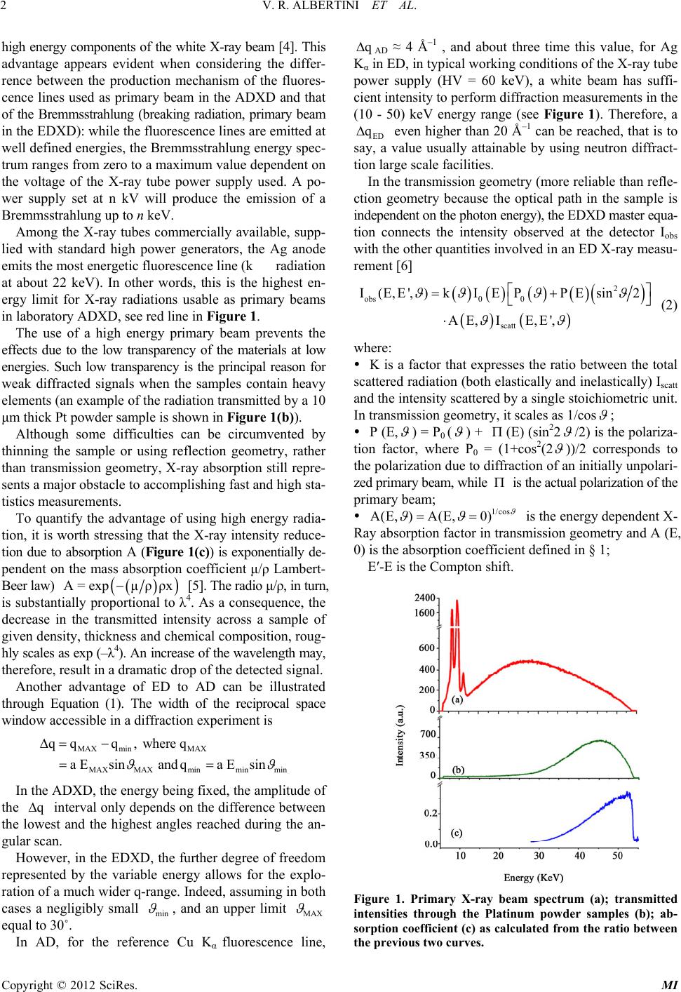 V. R. ALBERTINI ET AL. 2 high energy components of the white X-ray beam [4]. This advantage appears evident when considering the differ- rence between the production mechanism of the fluores- cence lines used as primary beam in the ADXD and that of the Bremmsstrahlung (breaking radiation, primary beam in the EDXD): while the fluorescence lines are emitted at well defined energies, the Bremmsstrahlung energy spec- trum ranges from zero to a maximum value dependent on the voltage of the X-ray tube power supply used. A po- wer supply set at n kV will produce the emission of a Bremmsstrahlung up to n keV. Among the X-ray tubes commercially available, supp- lied with standard high power generators, the Ag anode emits the most energetic fluorescence line (kradiation at about 22 keV). In other words, this is the highest en- ergy limit for X-ray radiations usable as primary beams in laboratory ADXD, see red line in Figure 1. The use of a high energy primary beam prevents the effects due to the low transparency of the materials at low energies. Such low transparency is the principal reason for weak diffracted signals when the samples contain heavy elements (an example of the radiation transmitted by a 10 μm thick Pt powder sample is shown in Figure 1(b)). Although some difficulties can be circumvented by thinning the sample or using reflection geometry, rather than transmission geometry, X-ray absorption still repre- sents a major obstacle to accomplishing fast and high sta- tistics measurements. To quantify the advantage of using high energy radia- tion, it is worth stressing that the X-ray intensity reduce- tion due to absorption A (Figure 1(c)) is exponentially de- pendent on the mass absorption coefficient μ/ρ Lambert- Beer law) A=exp μρρx [5]. The radio μ/ρ, in turn, is substantially proportional to λ4. As a consequence, the decrease in the transmitted intensity across a sample of given density, thickness and chemical composition, roug- hly scales as exp (–λ4). An increase of the wavelength may, therefore, result in a dramatic drop of the detected signal. Another advantage of ED to AD can be illustrated through Equation (1). The width of the reciprocal space window accessible in a diffraction experiment is MAX minMAX MAX MAXminmin min qqq, where q a Esinandqa Esin In the ADXD, the energy being fixed, the amplitude of the interval only depends on the difference between the lowest and the highest angles reached during the an- gular scan. q However, in the EDXD, the further degree of freedom represented by the variable energy allows for the explo- ration of a much wider q-range. Indeed, assuming in both cases a negligibly small min , and an upper limit MAX equal to 30˚. In AD, for the reference Cu Kα fluorescence line, q AD ≈ 4 Å–1 , and about three time this value, for Ag Kα in ED, in typical working conditions of the X-ray tube power supply (HV = 60 keV), a white beam has suffi- cient intensity to perform diffraction measurements in the (10 - 50) keV energy range (see Figure 1). Therefore, a ED q even higher than 20 Å–1 can be reached, that is to say, a value usually attainable by using neutron diffract- tion large scale facilities. In the transmission geometry (more reliable than refle- ction geometry because the optical path in the sample is independent on the photon energy), the EDXD master equa- tion connects the intensity observed at the detector Iobs with the other quantities involved in an ED X-ray measu- rement [6] 2 obs0 0 scatt I(E,E',)kIEPPEsin2 AE, IE,E', (2) where: K is a factor that expresses the ratio between the total scattered radiation (both elastically and inelastically) Iscatt and the intensity scattered by a single stoichiometric unit. In transmission geometry, it scales as 1/cos ; P (E, ) = P0 ( ) + (E) (sin22 /2) is the polariza- tion factor, where P0 = (1+cos2(2 ))/2 corresponds to the polarization due to diffraction of an initially unpolari- zed primary beam, while is the actual polarization of the primary beam; 1/cos A(E, )A(E,0) is the energy dependent X- Ray absorption factor in transmission geometry and A (E, 0) is the absorption coefficient defined in § 1; E′-E is the Compton shift. Figure 1. Primary X-ray beam spectrum (a); transmitted intensities through the Platinum powder samples (b); ab- sorption coefficient (c) as calculated from the ratio between the previous two curves. Copyright © 2012 SciRes. MI  V. R. ALBERTINI ET AL. 3 2. The Hybrid ED/AD X-Ray Diffraction Method The basic idea behind the method we propose is to take advantage of the merits of both the EDXD and the AD- XD by carrying out an ADXD-like measurements using an EDXD diffractometer. Therefore, from the operative point of view, the measurement is similar to the ordinary ADXD one, consisting of the collection of the diffracted intensity, from a minimum (0 ) to a maximum (n ) an- gular value, at steps of k = 0 + k with con- stant increment). The difference is that instead of an or- dinary monochromatic primary beam, like in a real AD- XD measurement, a polychromatic beam is used and the diffracted radiation is collected by an energy dispersive detector. As a consequence, at each k , a whole diffra- cttion pattern is acquired, instead of a single q-point as in the ADXD. A first merit of the hybrid method we propose is that, unlike the ADXD measurements, in which monochroma- tization imposes the suppression of all but the selected energy component, all the components are preserved and are collected in parallel, channel by channel (as in ED- XD). Therefore, the same technique adopted to draw an ADXD diffraction pattern, namely recording the intensity as a function of k , can be used here by plotting the in- tensity contained in each channel. To express this concept in formulas, we may say that, given a generic channel j (corresponding to an energy Ej), the diffraction pattern obtainable by plotting the number of photons contained in j as a function of k , is the cu- rve I vs. (Ej, k ), or rather, according to Equation (1), I (Ej·sin k ). Since all the channels can be used for this cal- culation, a number of diffraction patterns equal to the nu- mber of channels is obtained. Of course, for each choice of the energy Ej, the amplitude of the q-interval increases with k and its extremes shift towards higher values along the q axes. Indeed, the extremes of the q-interval can be expressed as: kminmink kMaxMax qa Esinandqa Esink (3) and, therefore, and , as well as the q-interval ( =–), increase with k kmin q kmin q kMax q k qkMax q . Such a procedure can be simplified to a certain extent, considering that, due to the finite energy resolution of the detector, adjacent channels are not independent. Thus, instead of analysing the intensity of every single channel, adjacent channels can be grouped and their collective intensity can be analysed altogether. Since the energy interval in our setup is 50 eV, while the energy resolution of the detector is about 200 eV, the channels can be grouped 5 by 5. All the diffraction patterns obtained in this way can be finally utilized (taking in account their relative q-shift) to compose an overall pattern that contains all the informa- tion present in each single pattern, as will be shown in the experimental section. 3. Hybrid ED/AD Measurements and Problems Connected to Data Correction and Refinement In Figures 2(a) and 2(b) the sequences of ED diffraction patterns collected as a function of k are shown in the form of 3D-maps. The maps refer to an Al and a Pt sample, respectively. They clearly exhibit the characteristics of diffraction in either ED or AD mode. The Bragg reflections appear in the (Ej, k ) plane as “crests”, and progressively shift to- wards lower energy values as k is increased (accord- ing to Equation (1), q = a·Ej·k sin ), following iso-q cu- rves. The crests intensity is modulated by the occurrence of phenomena concomitant to diffraction in an X-ray mea- surement, as will be discussed later. Vertical sections of the crests with planes parallel to the E axis are the energy dispersive patterns collected in correspondence of the -value at which the cutting plane is placed. Figure 2. Sequences of patterns (a) Aluminium; (b) Plati- num) collected as a function of energy and angle. The re- sulting crests represent the traces of Bragg reflections in their path along constant q-curves (approximately hyper- bolic) due to the angular scan. Copyright © 2012 SciRes. MI  V. R. ALBERTINI ET AL. 4 Conversely, vertical sections of the crests with planes parallel to the axis at a certain E-value, are equiva- lent to conventional AD patterns collected in correspond- dence of that E-value. Two planes of this kind at Ej = 40 keV and k = 15˚, respectively, are evidenced in Fi- gure 2(b) in red. First of all, we can make some general observations concerning these maps. Due to the low elec- tron number, the crests in Figure 2(a) span from low to medium q-values, being absent in the high q-zone becau- se of the rapid decrease of Al coherent form factor as a function of q. In contrast, in Figure 2(b), Pt crests are present also in the high q-zone, but their left tails tend to vanish as a consequence of the intense X-ray absorption in the low energy region. In such a region, the absorption gets even more intense with increasing angles, so that the left tails diminish faster at higher k . Secondly, on the basis of the master Equation (2), we can make a deeper preliminary inspection prior to data refinement. Let us take, for instance, the most intense peaks of Figure 2(a) and (b). Their intensities have maxima in the central part of the crests. This behavior is dominated by the three main factors influencing the height of Bragg reflections in the ED mode, namely, by the energy-de- pendent coefficients of Iscatt in Equation (2). At low ener- gies, both the primary beam intensity and the sample trans- parency are low, so that the peak amplitude lowers as well. At high energies, the transparency is high, but the inten- sity of the primary beam becomes vanishingly small, so that the result is, again, the decrease of the peak ampli- tude. In standard EDXD, these effects have to be taken into account and the data accurately corrected for them. Othe- rwise, major systematic errors, which produce profile di- stortions and make the measurement unreliable, occur [7]. For this reason, much effort has been dedicated to co- rrectly determine quantities that must be measured inde- pendently of the diffraction pattern collection. Unfortunately for the experimenter, such measurements are far from trivial, as discussed below. 3.1. Primary X-Ray Beam Spectrum, I0 (E) The determination of the primary beam spectrum is a pro- blem that dates back to the invention of the EDXD tech- nique [8]. The difficulty is due to the fact that a direct measurement of I0 is impossible because its high intensity “dazzles” the energy sensitive detector. Therefore, the tech- nique of measurement must be to collect a signal propor- tional to I0, but with a much lower intensity. Several ways have been suggested to do this, the most common being 1) an extreme collimation of the radiation; 2) the reduction of the X-ray tube power supply current; 3) the measure- ment of a rare gas scattering. 1) A high collimation reduces the beam cross section, and a direct acquisition of the incident beam becomes po- ssible by placing both the source and the detector arms in horizontal position [8]. However, two problems arise. The first is that, although the total photon flux is actually re- duced, the power density of the so-obtained thin beam is as high as in the original primary beam. This may produ- ce non-linear effects in the detector diode, where a high number of electron-hole couples are generated in a small volume per unit time. Furthermore, the collimation slits are partially transparent at high energies, so that the col- limated beam contains an extra-contribution in its upper part [9]. 2) The reduction of the power supply current to the re- gion of μA is also not perfectly reliable, since the focal spot on the anode may suffer unpredictable changes when the tube is forced to operate in such extreme conditions. Therefore, although theoretically a reduction of the cur- rent at a parity of high voltage should decrease the am- plitude of the energy spectrum leaving the profile shape unchanged, distortions must nevertheless be expected [9]. 3) Finally, the measurement of the scattering from a rare gas as Ar has been proposed [10]. This method is based on the simplification of the master equation when Ar is measured at small angles: 2 obs0 Ar IE, KIENfE, where N is the number of irradiated atoms and fAr is the coherent form factor. Indeed, the Compton scattering, at low angles and for a high atomic number sample, is neg- ligible; the cross (interatomic) interference term in a mo- noatomic gas is practically zero, as well as the absorption (due to low density). Furthermore, also the polarization disappears from the equation, because the measurement is accomplished at a fixed angle and the energy-depen- dent part is proportional to 2 sin 2 with small (Equa- tion (2)). Thus, 2 0obs IE IE,f Ar Nevertheless remarkable deviations from the theoretic- cal energy spectrum profile have also been observed in this case. 3.2. Polarization, P (E, ) The second problem concerns the determination of the primary beam polarization. It is well known that Brem- msstrahlung is polarized because, especially at high ene- rgies, the photons produced by the breaking of fast elec- trons tend to be emitted in a preferential direction, that is, in the direction of provenience of the electrons. In turn, the polarization of the scattered radiation is composed by two terms, P0 and (E), (see Equation (2)). The initial polarization (E) of the primary beam is extremely di- Copyright © 2012 SciRes. MI 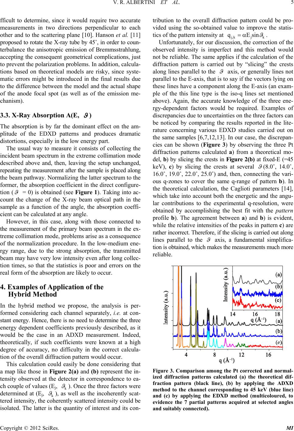 V. R. ALBERTINI ET AL. 5 fficult to determine, since it would require two accurate measurements in two directions perpendicular to each other and to the scattering plane [10]. Hanson et al. [11] proposed to rotate the X-ray tube by 45˚, in order to coun- terbalance the anisotropic emission of Bremmsstrahlung, accepting the consequent geometrical complications, just to prevent the polarization problems. In addition, calcula- tions based on theoretical models are risky, since syste- matic errors might be introduced in the final results due to the difference between the model and the actual shape of the anode focal spot (as well as of the emission me- chanism). 3.3. X-Ray Absorption A(E, ) The absorption is by far the dominant effect on the am- plitude of the EDXD patterns and produces dramatic distortions, especially in the low energy part. The usual way to measure it consists of collecting the incident beam spectrum in the extreme collimation mode described above and, then, leaving the setup unchanged, repeating the measurement after the sample is placed along the beam pathway. Normalizing the latter spectrum to the former, the absorption coefficient in the direct configure- tion ( = 0) is obtained (see Figure 1). Taking into ac- count the change of the X-ray beam optical path in the sample as a function of the angle, the absorption coeffi- cient can be calculated at any angle. However, in this case, along with those connected to the measurement of the primary beam spectrum in the ex- treme collimation mode, problems arise as a consequence of the normalization procedure. In the low-medium ene- rgy range, due to the strong absorption, the transmitted beam may have very low intensity even after long collec- tion times, so that the statistics is poor and errors on the real form of the absorption are likely to occur. 4. Examples of Application of the Hybrid Method In the hybrid method we propose, the analysis is per- formed considering each channel separately, i.e. at con- stant energy. Hence, there is no need to determine the three energy dependent coefficients previously described, as it would be the case in an ADXD measurement. Indeed, theoretically, if such coefficients were known at a high degree of accuracy, no difficulty in the correct calcula- tion of the overall diffraction pattern would occur. This calculation could easily be done considering that a map like those in Figure 2(a) and (b) represent the in- tensity observed at the detector in correspondence to ea- ch couple of values (Ej, k ). Once the three factors were determined at (Ej, k ), as well as the incoherently scat- tered intensity, the coherently scattered intensity could be isolated. The latter is the quantity of interest and its con- tribution to the overall diffraction pattern could be pro- vided using the so-obtained value to improve the statis- tics of the pattern intensity at j,kj k qEsin . Unfortunately, for our discussion, the correction of the observed intensity is imperfect and this method would not be reliable. The same applies if the calculation of the diffraction pattern is carried out by “slicing” the crests along lines parallel to the axis, or generally lines not parallel to the E-axis, that is to say if the vectors lying on these lines have a component along the E-axis (an exam- ple of the this line type is the iso-q lines set mentioned above). Again, the accurate knowledge of the three ene- rgy-dependent factors would be required. Examples of discrepancies due to uncertainties on the three factors can be noticed by comparing the results reported in the lite- rature concerning various EDXD studies carried out on the same samples [6,7,12,13]. In our case, the discrepan- cies can be shown (Figure 3) by observing the three Pt diffraction patterns calculated a) from a theoretical mo- del, b) by slicing the crests in Figure 2(b) at fixed-E (=45 keV), c) by slicing the crests at several (8.0˚, 14.0˚, 16.0˚, 19.0˚, 22.0˚, 25.0˚) and, then, connecting the vari- ous q-zones to cover the same q-range of pattern b). In the theoretical calculation, the Caglioti parameters [14], which take into account both the energetic and the angu- lar contributions to the experimental q-resolution, were obtained by accomplishing the best fit with the pattern profile b). The agreement between a) and b) is evident, while the relative intensities of the peaks in pattern c) are rather incorrect. Therefore, if the slicing is carried out along lines parallel to the axis, a fundamental simplifica- tion is obtained, which makes the measurements much more reliable. Figure 3. Comparison among the Pt corrected and normal- ized diffraction patterns calculated (a) the theoretical dif- fraction pattern (black line), (b) by applying the ADXD method to the channel corresponding to 45 keV (blue line) and (c) by applying the EDXD method (multicoloured, to evidence the 7 partial patterns acquired at selected angles and suitably connected). Copyright © 2012 SciRes. MI 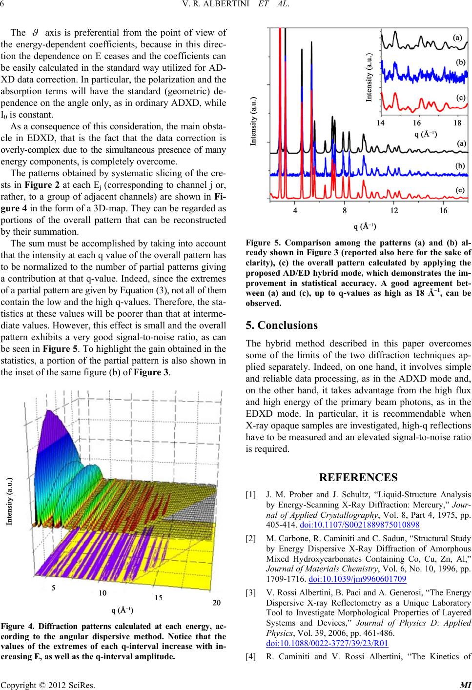 V. R. ALBERTINI ET AL. 6 The axis is preferential from the point of view of the energy-dependent coefficients, because in this direc- tion the dependence on E ceases and the coefficients can be easily calculated in the standard way utilized for AD- XD data correction. In particular, the polarization and the absorption terms will have the standard (geometric) de- pendence on the angle only, as in ordinary ADXD, while I0 is constant. As a consequence of this consideration, the main obsta- cle in EDXD, that is the fact that the data correction is overly-complex due to the simultaneous presence of many energy components, is completely overcome. The patterns obtained by systematic slicing of the cre- sts in Figure 2 at each Ej (corresponding to channel j or, rather, to a group of adjacent channels) are shown in Fi- gure 4 in the form of a 3D-map. They can be regarded as portions of the overall pattern that can be reconstructed by their summation. The sum must be accomplished by taking into account that the intensity at each q value of the overall pattern has to be normalized to the number of partial patterns giving a contribution at that q-value. Indeed, since the extremes of a partial pattern are given by Equation (3), not all of them contain the low and the high q-values. Therefore, the sta- tistics at these values will be poorer than that at interme- diate values. However, this effect is small and the overall pattern exhibits a very good signal-to-noise ratio, as can be seen in Figure 5. To highlight the gain obtained in the statistics, a portion of the partial pattern is also shown in the inset of the same figure (b) of Figure 3. Figure 4. Diffraction patterns calculated at each energy, ac- cording to the angular dispersive method. Notice that the values of the extremes of each q-interval increase with in- creasing E, as well as the q-interval amplitude. Figure 5. Comparison among the patterns (a) and (b) al- ready shown in Figure 3 (reported also here for the sake of clarity), (c) the overall pattern calculated by applying the proposed AD/ED hybr id mode, which demonstrates the im- provement in statistical accuracy. A good agreement bet- ween (a) and (c), up to q-values as high as 18 Å–1, can be observed. 5. Conclusions The hybrid method described in this paper overcomes some of the limits of the two diffraction techniques ap- plied separately. Indeed, on one hand, it involves simple and reliable data processing, as in the ADXD mode and, on the other hand, it takes advantage from the high flux and high energy of the primary beam photons, as in the EDXD mode. In particular, it is recommendable when X-ray opaque samples are investigated, high-q reflections have to be measured and an elevated signal-to-noise ratio is required. REFERENCES [1] J. M. Prober and J. Schultz, “Liquid-Structure Analysis by Energy-Scanning X-Ray Diffraction: Mercury,” Jour- nal of Applied Crystallography, Vol. 8, Part 4, 1975, pp. 405-414. doi:10.1107/S0021889875010898 [2] M. Carbone, R. Caminiti and C. Sadun, “Structural Study by Energy Dispersive X-Ray Diffraction of Amorphous Mixed Hydroxycarbonates Containing Co, Cu, Zn, Al,” Journal of Materials Chemistry, Vol. 6, No. 10, 1996, pp. 1709-1716. doi:10.1039/jm9960601709 [3] V. Rossi Albertini, B. Paci and A. Generosi, “The Energy Dispersive X-ray Reflectometry as a Unique Laboratory Tool to Investigate Morphological Properties of Layered Systems and Devices,” Journal of Physics D: Applied Physics, Vol. 39, 2006, pp. 461-486. doi:10.1088/0022-3727/39/23/R01 [4] R. Caminiti and V. Rossi Albertini, “The Kinetics of Copyright © 2012 SciRes. MI 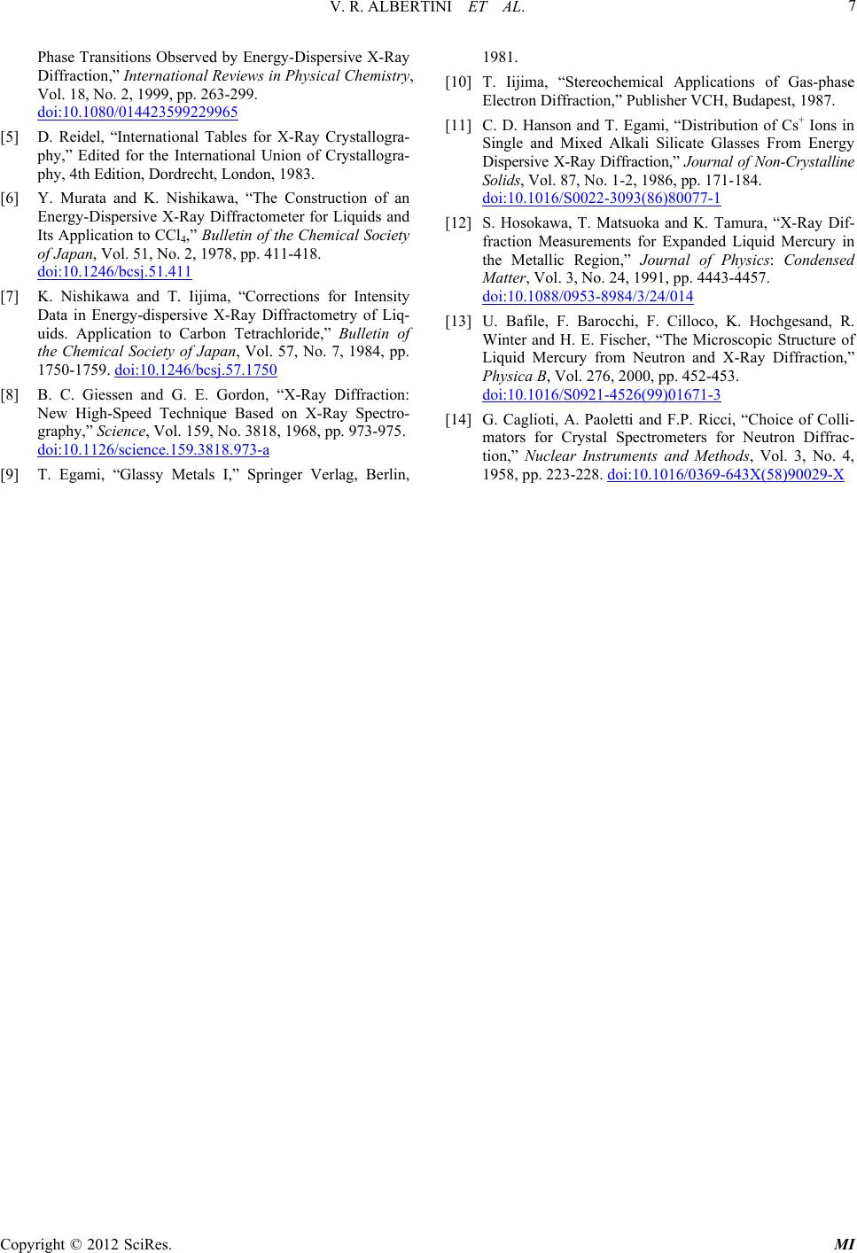 V. R. ALBERTINI ET AL. Copyright © 2012 SciRes. MI 7 Phase Transitions Observed by Energy-Dispersive X-Ray Diffraction,” International Reviews in Physical Chemistry, Vol. 18, No. 2, 1999, pp. 263-299. doi:10.1080/014423599229965 [5] D. Reidel, “International Tables for X-Ray Crystallogra- phy,” Edited for the International Union of Crystallogra- phy, 4th Edition, Dordrecht, London, 1983. [6] Y. Murata and K. Nishikawa, “The Construction of an Energy-Dispersive X-Ray Diffractometer for Liquids and Its Application to CCl4,” Bulletin of the Chemical Society of Japan, Vol. 51, No. 2, 1978, pp. 411-418. doi:10.1246/bcsj.51.411 [7] K. Nishikawa and T. Iijima, “Corrections for Intensity Data in Energy-dispersive X-Ray Diffractometry of Liq- uids. Application to Carbon Tetrachloride,” Bulletin of the Chemical Society of Japan, Vol. 57, No. 7, 1984, pp. 1750-1759. doi:10.1246/bcsj.57.1750 [8] B. C. Giessen and G. E. Gordon, “X-Ray Diffraction: New High-Speed Technique Based on X-Ray Spectro- graphy,” Science, Vol. 159, No. 3818, 1968, pp. 973-975. doi:10.1126/science.159.3818.973-a [9] T. Egami, “Glassy Metals I,” Springer Verlag, Berlin, 1981. [10] T. Iijima, “Stereochemical Applications of Gas-phase Electron Diffraction,” Publisher VCH, Budapest, 1987. [11] C. D. Hanson and T. Egami, “Distribution of Cs+ Ions in Single and Mixed Alkali Silicate Glasses From Energy Dispersive X-Ray Diffraction,” Journal of Non-Crystalline Solids, Vol. 87, No. 1-2, 1986, pp. 171-184. doi:10.1016/S0022-3093(86)80077-1 [12] S. Hosokawa, T. Matsuoka and K. Tamura, “X-Ray Dif- fraction Measurements for Expanded Liquid Mercury in the Metallic Region,” Journal of Physics: Condensed Matter, Vol. 3, No. 24, 1991, pp. 4443-4457. doi:10.1088/0953-8984/3/24/014 [13] U. Bafile, F. Barocchi, F. Cilloco, K. Hochgesand, R. Winter and H. E. Fischer, “The Microscopic Structure of Liquid Mercury from Neutron and X-Ray Diffraction,” Physica B, Vol. 276, 2000, pp. 452-453. doi:10.1016/S0921-4526(99)01671-3 [14] G. Caglioti, A. Paoletti and F.P. Ricci, “Choice of Colli- mators for Crystal Spectrometers for Neutron Diffrac- tion,” Nuclear Instruments and Methods, Vol. 3, No. 4, 1958, pp. 223-228. doi:10.1016/0369-643X(58)90029-X
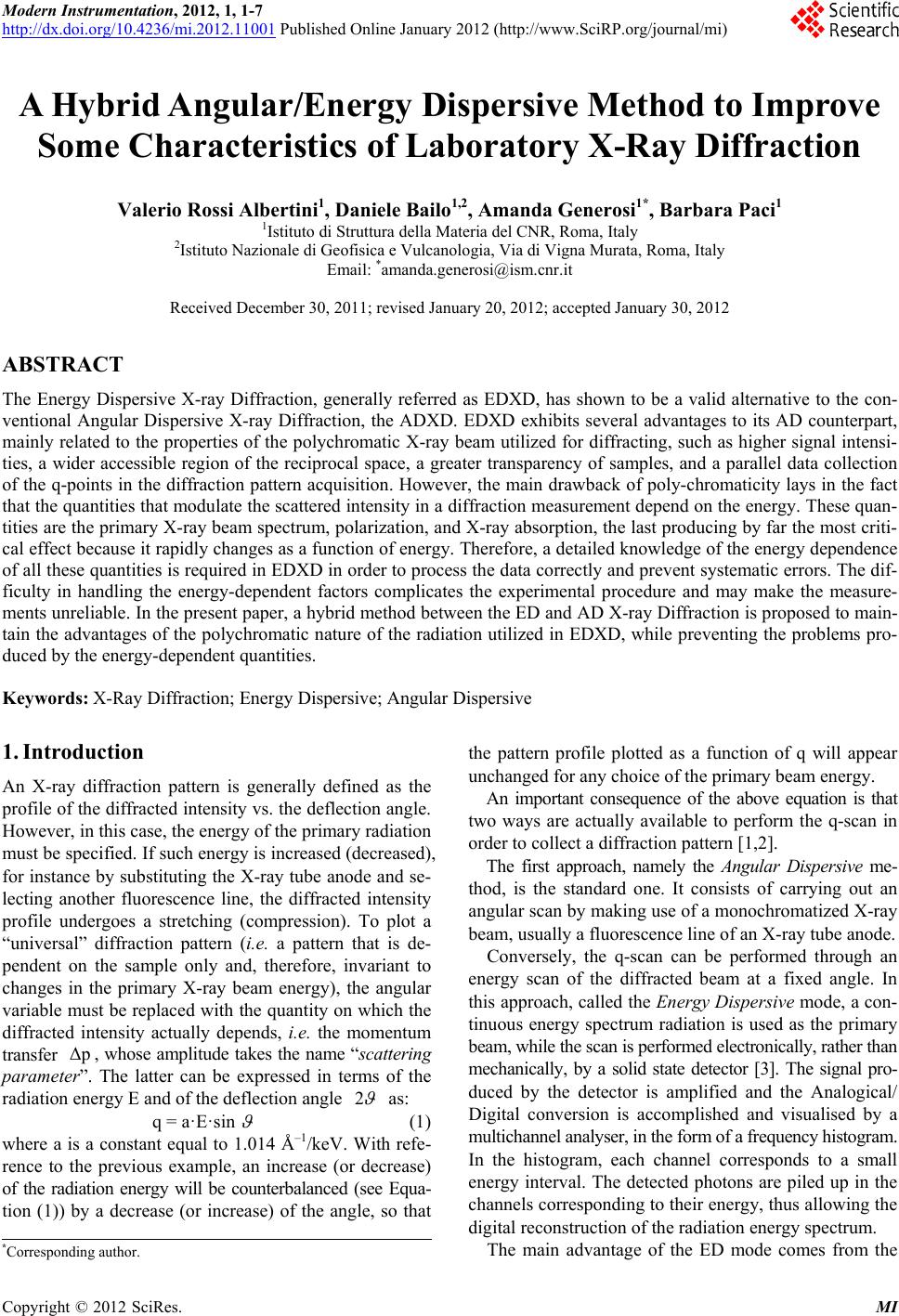
|