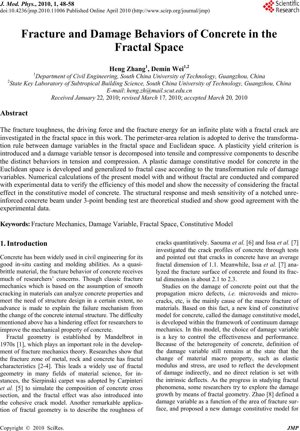J. Mod. Phys., 2010, 1, 48-58
doi:10.4236/jmp.2010.11006 Published Online April 2010 (http://www.scirp.org/journal/jmp)
Fracture and Damage Behaviors of Concrete in the
Fractal Space
Heng Zhang1, Demin Wei1,2
1Department of Civil Engineering, South China University of Technology, Guangzhou, China
2State Key Laboratory of Subtropical Building Science, South China University of Technology, Guangzhou, China
Received January 22, 2010; revised March 17, 2010; accepted March 20, 2010
Abstract
The fracture toughness, the driving force and the fracture energy for an infinite plate with a fractal crack are
investigated in the fractal space in this work. The perimeter-area relation is adopted to derive the transforma-
tion rule between damage variables in the fractal space and Euclidean space. A plasticity yield criterion is
introduced and a damage variable tensor is decomposed into tensile and compressive components to describe
the distinct behaviors in tension and compression. A plastic damage constitutive model for concrete in the
Euclidean space is developed and generalized to fractal case according to the transformation rule of damage
variables. Numerical calculations of the present model with and without fractal are conducted and compared
with experimental data to verify the efficiency of this model and show the necessity of considering the fractal
effect in the constitutive model of concrete. The structural response and mesh sensitivity of a notched unre-
inforced concrete beam under 3-point bending test are theoretical studied and show good agreement with the
experimental data.
Keywords: Fracture Mechanics, Damage Variable, Fractal Space, Constitutive Model
1. Introduction
Concrete has been widely used in civil engineering for its
good in-situ casting and molding abilities. As a quasi-
brittle material, the fracture behavior of concrete receives
much of researchers’ concerns. Though classic fracture
mechanics which is based on the assumption of smooth
cracking in materials can analyze concrete properties and
meet the need of structure design in a certain extent, no
advance is made to explain the failure mechanism from
the change of the concrete internal structure. The difficulty
mentioned above has a hindering effect for researchers to
improve the mechanical property of concrete.
Fractal geometry is established by Mandelbrot in
1970s [1], which plays an important role in the develop-
ment of fracture mechanics theory. Researches show that
the fracture zone of metal, rock and concrete has fractal
characteristics [2-4]. This leads a widely use of fractal
geometry in many fields of material science, for in-
stances, the Sierpinski carpet was adopted by Carpinteri
et al. [5] to simulate the composition of concrete cross
section, and the fractal effect was also introduced into
the cohesive crack model. Another remarkable applica-
tion of fractal geometry is to describe the roughness of
cracks quantitatively. Saouma et al. [6] and Issa et al. [7]
investigated the crack profiles of concrete through tests
and pointed out that cracks in concrete have an average
fractal dimension of 1.1. Meanwhile, Issa et al. [7] ana-
lyzed the fracture surface of concrete and found its frac-
tal dimension is about 2.1 to 2.3.
Studies on the damage of concrete point out that the
propagation micro defects, i.e. microvoids and micro-
cracks, etc, is the mainly cause of the macro fracture of
materials. Based on this fact, a new kind of constitutive
model for concrete, called the damage constitutive model,
is developed within the framework of continuum damage
mechanics. In this model, the choice of damage variable
is a key to control the effectiveness and performance.
Because of the heterogeneity of concrete, definition of
the damage variable still remains at the state that the
change of material macro property, such as elastic
modulus and stress, are used to reflect the development
of damage indirectly, and no direct relation is set with
the intrinsic deflects. As the progress in studying fractal
phenomena, some researchers try to explore the damage
growth by means of fractal geometry. Zhao [8] defined a
damage variable as a function of the area of fracture sur-
face, and proposed a new damage constitutive model for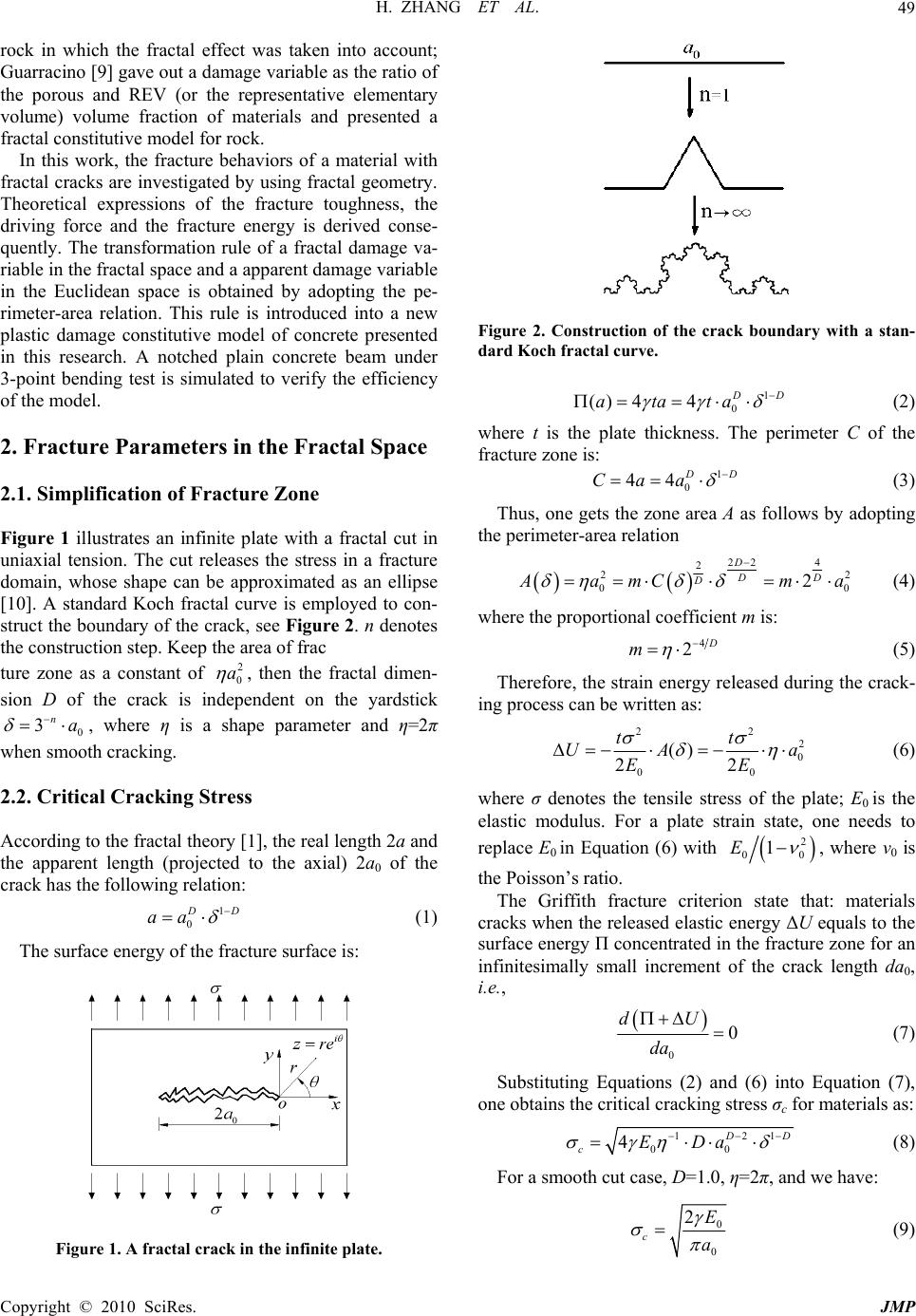

H. ZHANG ET AL. 49
rock in which the fractal effect was taken into account;
Guarracino [9] gave out a damage variable as the ratio of
the porous and REV (or the representative elementary
volume) volume fraction of materials and presented a
fractal constitutive model for rock.
In this work, the fracture behaviors of a material with
fractal cracks are investigated by using fractal geometry.
Theoretical expressions of the fracture toughness, the
driving force and the fracture energy is derived conse-
quently. The transformation rule of a fractal damage va-
riable in the fractal space and a apparent damage variable
in the Euclidean space is obtained by adopting the pe-
rimeter-area relation. This rule is introduced into a new
plastic damage constitutive model of concrete presented
in this research. A notched plain concrete beam under
3-point bending test is simulated to verify the efficiency
of the model.
2. Fracture Parameters in the Fractal Space
2.1. Simplification of Fracture Zone
Figure 1 illustrates an infinite plate with a fractal cut in
uniaxial tension. The cut releases the stress in a fracture
domain, whose shape can be approximated as an ellipse
[10]. A standard Koch fractal curve is employed to con-
struct the boundary of the crack, see Figure 2. n denotes
the construction step. Keep the area of frac
ture zone as a constant of 2
0
a

, then the fractal dimen-
sion D of the crack is independent on the yardstick
0
3na 

, where η is a shape parameter and η=2π
when smooth cracking.
2.2. Critical Cracking Stress
According to the fractal theory [1], the real length 2a and
the apparent length (projected to the axial) 2a0 of the
crack has the following relation:
1
0
D
D
aa


 (1)
The surface energy of the fracture surface is:
Figure 1. A fractal crack in the infinite plate.
Figure 2. Construction of the crack boundary with a stan-
dard Koch fractal curve.
1
0
() 44
D
D
atata



  (2)
where t is the plate thickness. The perimeter C of the
fracture zone is:
1
0
44
D
D
Caa


 (3)
Thus, one gets the zone area A as follows by adopting
the perimeter-area relation
 
22 4
2
22
00
2
D
DD
D
A
amCm a  


  (4)
where the proportional coefficient m is:
4
2
D
m 

 (5)
Therefore, the strain energy released during the crack-
ing process can be written as:
22
2
0
00
()
22
tt
UA a
EE



  (6)
where σ denotes the tensile stress of the plate; E0 is the
elastic modulus. For a plate strain state, one needs to
replace E0 in Equation (6) with

2
00
1E

, where ν0 is
the Poisson’s ratio.
The Griffith fracture criterion state that: materials
cracks when the released elastic energy ΔU equals to the
surface energy Π concentrated in the fracture zone for an
infinitesimally small increment of the crack length da0,
i.e.,


0
0
dU
da
  (7)
Substituting Equations (2) and (6) into Equation (7),
one obtains the critical cracking stress σc for materials as:
121
00
4
D
D
cEDa
 

 (8)
For a smooth cut case, D=1.0, η=2π, and we have:
0
0
2
c
E
a

  (9)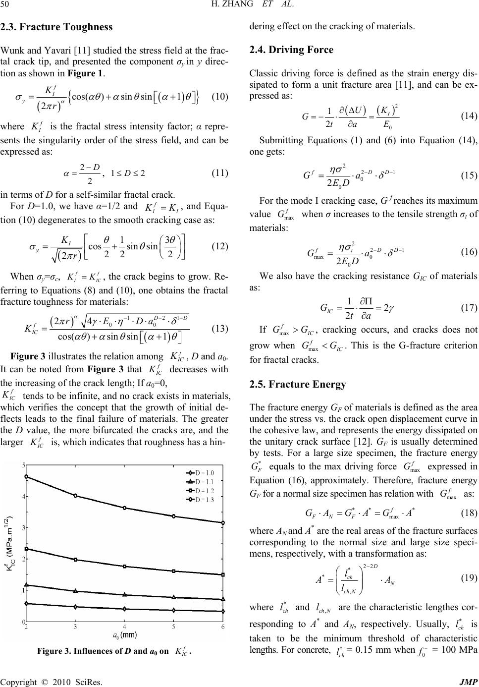

H. ZHANG ET AL. 50
2.3. Fracture Toughness
Wunk and Yavari [11] studied the stress field at the frac-
tal crack tip, and presented the component σy in y direc-
tion as shown in Figure 1.
 

cos()sinsin1
2
f
I
y
K
r


 

 

(10)
where f
I
K
is the fractal stress intensity factor; α repre-
sents the singularity order of the stress field, and can be
expressed as:
2
2
D


, 12D (11)
in terms of D for a self-similar fractal crack.
For D=1.0, we have α=1/2 and f
I
I
KK, and Equa-
tion (10) degenerates to the smooth cracking case as:

13
cossin sin
22 2
2
I
y
K
r







 


(12)
When σy=σc, ff
I
IC
K
K, the crack begins to grow. Re-
ferring to Equations (8) and (10), one obtains the fractal
fracture toughness for materials:


121
00
24
cos()sinsin1
D
D
f
IC
rEDa
K

 
 

 



(13)
Figure 3 illustrates the relation among
f
I
C
K
, D and a0.
It can be noted from Figure 3 that
f
I
C
K decreases with
the increasing of the crack length; If a0=0,
f
I
C
K tends to be infinite, and no crack exists in materials,
which verifies the concept that the growth of initial de-
flects leads to the final failure of materials. The greater
the D value, the more bifurcated the cracks are, and the
larger
f
I
C
K is, which indicates that roughness has a hin-
Figure 3. Influences of D and a0 on
f
I
C
K
.
dering effect on the cracking of materials.
2.4. Driving Force
Classic driving force is defined as the strain energy dis-
sipated to form a unit fracture area [11], and can be ex-
pressed as:

2
0
1
2
I
UK
Gta E

 
 (14)
Submitting Equations (1) and (6) into Equation (14),
one gets:
2
21
0
0
2
fDD
Ga
ED



 (15)
For the mode I cracking case, G f reaches its maximum
value max
f
G when σ increases to the tensile strength σt of
materials:
2
21
max 0
0
2
fDD t
Ga
ED




(16)
We also have the cracking resistance GIC of materials
as:
12
2
IC
Gta


 
 (17)
If max
f
I
C
GG, cracking occurs, and cracks does not
grow when max
f
I
C
GG. This is the G-fracture criterion
for fractal cracks.
2.5. Fracture Energy
The fracture energy GF of materials is defined as the area
under the stress vs. the crack open displacement curve in
the cohesive law, and represents the energy dissipated on
the unitary crack surface [12]. GF is usually determined
by tests. For a large size specimen, the fracture energy
*
F
G equals to the max driving force max
f
G expressed in
Equation (16), approximately. Therefore, fracture energy
GF for a normal size specimen has relation with max
f
G as:
** *
max
f
FN F
GAGA GA

  (18)
where AN and A* are the real areas of the fracture surfaces
corresponding to the normal size and large size speci-
mens, respectively, with a transformation as:
22
*
*
,
D
ch
N
ch N
l
A
A
l







(19)
where *
ch
l and ,ch N l are the characteristic lengthes cor-
responding to A* and AN, respectively. Usually, *
ch
l is
taken to be the minimum threshold of characteristic
lengths. For concrete, *
ch
l= 0.15 mm when0
f
 = 100 MPa

H. ZHANG ET AL. 51
and *
ch
l= 0.15 mm when 0
f

= 200 MPa [13], and *
ch
l
can be obtained by linear interpolation for other strengths.
,ch N
l is given by [14]:
,0
2
ch N
lab (20)
where the constant b < 1 represents the initially cracked
portion of the interface prior to load application, 2a0 is
the initial crack diameter and is assumed to be equal to
the maximum aggregate size in concrete.
Substituting Equations (16) and (19) into Equation
(18), one obtains
22 2
,21
0
*
0
2
D
ch NDD
t
F
ch
l
Ga
ED l







 (21)
Here 2a0 needs is considered to be the final length of
the main crack for concrete, and represents a specimen
size. Figure 4 shows the behaviors of GF as the changes
of a0 and D. We can find that GF increases with the in-
creasing of these two factors.
3. Damage Variable
An apparent damage variable is defined as the ratio of
the effective bearing area Ak and the cross section area Ac
of materials, and has the following form:
k
c
A
A
  (22)
For a Euclidean shape, the area A0 and the perimeter
C0 have the following relation:
2
000
A
mC (23)
where m0 is a shape constant. Substituting Equation (23)
into Equation (22), one obtains the expression for the
apparent damage variable

as follows:
and
2
k
c
C
C




(24)
where Ck and Cc are the perimeters corresponding to Ak
and Ac, respectively. It is reasonable for us to take Ck
Figure 4. Influences of D and a0 on GF.
Cc as the crack length in one direction and the total
length of all cracks in all directions in a unit cell at fail-
ure, respectively.
By referring to Equation (1), the perimeter C of a
fractal damaged surface and the counterpart C0 in the
Euclidean space has the following relation:
1
0
D
D
ch
CCl

 (25)
Substituting Equation (4) into Equation (22), concern-
ing Equation (25), and based on the fact that cracks in
concrete is statistically self-similar fractal when the
yardstick δ ranges from 0.263 to 1 [15], one obtains the
following expression for a fractal damage variable in the
fractal space:
11
ˆ16 ck
DD








 (26)
where Dk = 1.0 ~ 2.0. From Equation (29), we find that
only the fractal dimension is different between the fractal
and apparent damage variables, and δ has no influence
on this relation. Since Ac is the cross section area of ma-
terials, which indicates Dc = 1.0, thus Equation (26) can
be rewritten as:
1
1
ˆ16 k
D
ij ij








 (27)
For a smooth crack, Dk = 1.0, and no fractal effect ex-
ists, and we have:
ˆij ij



(28)
From the above discussion, we notice that the apparent
damage variable in the Euclidean space is a special case
of the fractal damage variable in the fractal space, and
the fractal damage variable is the generalization of the
apparent damage variable. Figure 5 illustrates the dif-
ferences between the two kind damage variables in uni-
axial compression with an assumption that Dk takes the
average value of 1.1, and the original evolution data for
apparent damage variables is referred from reference
[16].
Figure 5. Evolutions of damage variables for concrete in
uniaxial compression cases.

H. ZHANG ET AL. 52
4. Plastic Damage Constitutive Model for
Concrete
Among the various existed constitutive models for con-
crete, the plastic damage model has a better effect to
characterize the stiffness degeneration, the strain soften-
ing and the unilateral effect of concrete under various
loading conditions.
4.1. Decomposition of Effective Stress Tensor
In view of the fact that the typical failure modes of con-
crete are cracking in tension and crushing in compression,
we decompose the effective stress tensor into tensile and
compressive parts (denoted by  σ and  σ, respec-
tively) by utilizing spectral decomposition technique
[17,18]:
:

σPσ (29)
:

 
+
σσσPσ (30)
where P+ and P- are the fourth-order projection tensors
expressed as [19]:

iii ii
i
H 


Ppp (31)

PIP (32)
where I is the fourth-order identity tensor;


i
H

represents the Heaviside function calculated for the ith
eigenvalue i

of σ; Pij is the second-order tensor and
is defined as:

1
2
ijjiij ji
 pp nnnn (33)
where ni is the ith normalized eigenvector corresponding
to i

.
4.2. Plasticity
We adopt a plasticity yield function f and a plastic poten-
tial function Fp as:
 
 12 max
ˆ
,3 fIJ   σκκ



10c 

 κ (34)
21
3
pp
F
JI   (35)
where

2xxx denotes the Macaulay bracket
function, max
ˆ

is the algebraically maximum effective
principal stress. α, β and c are parameters with the fol-
lowing forms [20]:
00
00
2
b
b
f
f
f
f




;



11
c
c





κ
κ


cf

κκ;



cf

κκ (36)
where 0b
f

and 0
f

are the initial equibiaxial and uni-
axial compressive yield stresses, respectively. 00b
f
f


lies between 1.10 and 1.20 from experiments, therefore,
α varies from 0.08 to 0.12.

cκ represent the inner
cohesion, and


fκ are the evolution stresses (posi-
tive values are used here in compression) in the effective
stress space due to plastic hardening or softening under
uniaxial tension and compression, respectively. 1
I
is
the first invariant of the effective stress tensor, 2
J
is
the second invariant of the effective deviatoric stress
tensor. αp ≥ 0 is a dilation parameter with 0.2 ≤ αp ≤ 0.3
for concrete.
According to the flow rule, the rate of the effective
plastic strain
p

 can be written as:
2
3
23
p
ij
pp pp
ij ij
ij
s
F
J

 



 


  (37)
where
p

 is a plastic consistency factor, and can be
determined by the consistency condition for the yield
surface f, which can be expressed in the Kuhn-Tucker
form as:
0f

, 0
p
 
, 0
pf
 
, 0
pf
 
  (38)
In this study, the linear isotropic hardening rules are
introduced to describe the change of the yield surfaces in
the effective stress space, and can be expressed in simple
forms as [21]:


p
y
ffE 


κ (39)
where y
f

are the effective yield strengths in uniaxial
tension and compression, and have approximate values
as 0y
f
f


 and0y
f
f


, respectively. 0
f

are the
uniaxial yield strengths of concrete corresponding to
tension and compression, respectively. p E

are the
effective plastic hardening modulus in uniaxial case, and
have relation with the elastoplastic tangent modulus
ep
E

as [22]:
0
0
ep
p
ep
EE
EEE



 (40)
According to the plasticity consistency condition, we
have:
0
ff
f



σκ
σκ
 (41)
and obtain the rate form of the constitutive equation as
follows:
0,
p
p
ijijkl kl
kl
F
C 







   (42)
where C0,ijkl is the fourth-order undamaged elastic stiff-

H. ZHANG ET AL. 53
ness tensor.
Accounting for the coupling of tension and compres-
sion, κ
 can be written as [22]:

max min
,(1)T
pp
ww  κ
 
(43)
where max
p

 and min
p

 are the maximum and minimum
values of the equivalent plastic strains
p
ij

; w is the
weight factor and has the following form:
33
11
ˆˆ
ii
ii
w



 (44)
where ˆi

are the principle stresses.
Substituting Equations (42) and (43) into Equation
(41), we obtain:
0,
1
p
ijkl kl
p
ij
fC
h







 (45)
where
p
h can be expressed in the following forms:
0,
max
ˆ
p
p
p
ijkl
ij kl
f
FfF
hC w
 


 

  (46)

0,
min
1ˆ
p
p
p
ijkl
ij kl
f
FfF
hC w
 


 

  (47)
where max
ˆ

and min
ˆ

are the maximum and minimum
effective principle stresses, respectively. Therefore, we
can rewrite the rate form of the relation Equation (42) for
the effective stress and the strain as:
ijijkl kl
C

 
 (48)
where Cijkl is the elasto-plastic tangent stiffness tensor
and has the following form:
0, 0,0,
1p
ijkl ijklijrsmnkl
p
rs mn
Ff
CC CC
h


  (49)
4.3. Helmholtz Free Energy
A damage constitutive model of a material is based on
the second law of thermodynamics which states that all
the selected internal variables must satisfy the Clau-
sius-Duhem inequality for any irreversible process under
an isothermal condition, and has a simple form as:
:0

σε 
 (50)
where σ and ε are the stress and strain tensors,

is the
total Helmholtz free energy (HFE) which can be consid-
ered as the sum of the elastic part e

and the plastic
part
p

, that is:


,,, ,
eeep
 εκΦεΦ κΦ
(51)
where Φ is the damage variable tensor.
We decompose e

into tensile and compressive
parts as:
 
,,,
eee ee e


εΦεε (52)
where

0
1
,11:
2
eee eee
 
 
 εεσε (53)

0
1
,11 :
2
ee eee
 
 
εεσε (54)
where




0:2
ee e


εσε represent the initial elastic
strain energy of materials;

 are the tensile and com-
pressive components of Φ. Therefore, we derive:



00
11
ee ee
ee





 

εε
σ
εε


11 


 σσ (55)
The incremental form of Equation (55) can be ex-
pressed as:




11 dd 


 
+
σσ σσσ


 (56)
Equations (56) and (48) form the final plastic damage
constitutive equations for the plain concrete.
Similarly, we can rewrite
p

as:




,, ,
pp p



κκ κ (57)
Referring to the fact that the contribution to the plastic
HFE from plastic strains of concrete in tension is much
smaller comparing to the one in compression, we assume
that 0
p



. Thus, we have:






0
,1
ppp


κκ κ (58)
Substituting Equations (51), (52) and (58) into Equa-
tion (50), we get:
:0
ep
ep
e

  

 
 

 
σεσεκΦ
κΦε

  (59)
Since the above inequality must be satisfied for any
elastic strain εe, we have:
e
e




σ
ε (60)
0YΦ
 (61)
:0
p
p
 



σε κ
κ
  (62)
where Y is the damage energy release rate and can be
expressed as:




YΦ (63)
According to the above discussions about the total
HFE, we can rewrite Y as:
0
Y



 (64)

H. ZHANG ET AL. 54
We define the damage criteria in tension and compres-
sion for concrete, respectively, as:

,0gYrY r
 
 (65)
where r are the current damage thresholds whose ini-
tial values is denoted by 0 r. Equation (65) indicates that
damage is initiated when Y exceed the corresponding
damage thresholds r.
Initial strain energy of materials can be written as:

00 0
1::0
2
eee ee


 εεεCε (66)


00 0
ee p

 
εκ （67)
where 0
e

 is the initial strain energy of materials in
compression, and can be expressed as:
 
2
0
0021011
0
12
121 0
23
eJIII
E

 



 


(68)

021211
1
62
23
p
pp
J
IJ II








κ
s

212 11
0
1
62
26
p
J
IJ II
E

 




(69)
where 2
:2
J
sss is the norm of s;
2
1:
2
J
ss is the second invariant of the compres-
sive effective deviatoric stress tensor  s; 1 I and 1 I

are the first invariant of

σ and  σ, respectively.
0
2p E 

 s
 is a material parameter.
Therefore, 0

 has the following form in compres-
sion case:

2
00211 221311
32
J
IJ III 
 

 


(70)
where parameters Ω0, Ω1, Ω2, Ω3 are

0
0
0
621
6E

 
 ;

1
0
3
621
p



  

0
2
0
12
621



  ;

0
3
0
0.5 3
621



   (71)
Assume that concrete is in biaxial compression, which
indicates σ3≡0, and we have:


22 0
012 12
00
22
121212
0
66 63
66
6
6
p
YEE
E


 
 
 

 


(72)
For an uniaxial compression case, we denote the uni-
axial compressive ultimate strength as 0 f, and have
σ1=0
f

,σ2=0. We can derive the initial damage threshold
0
r

as:


0
0
0
361
6
p
f
rE 






 (73)
And for an equibiaxial compression case, we use 0b
f

to denote the biaxial compressive ultimate strength. One
gets σ1=σ2=0b
f

, and derives 0 r as:




0
00
0
6161 2
6
bp
f
rE 






 (74)
Noticing that the initial damage threshold is unique for
a material, we obtain the expression for Ω from Equa-
tions (73) and (74):



2
000
2
00
61 3
6161 2
b
p
p
b
ff
ff






  (75)
For concrete, one has 00b
f
f

 = 1.10~1.16 and
p

=
0.2~0.3. Assuming ν0=0.2, and substituting the above
three parameters into Equation (74), we find that Ω ≥ 0 is
always hold. Thus we have 0
p

≥0 (see Equation (69)),
and 000
ep
Y




 ≥0, and finally have Y

≥0.
Accounting for the fact that damage is irreversible, we
get


,


≥ 0. Therefore, the total HFE defined in
Equation (51) satisfies the thermodynamic consistency,
or satisfies the inequality of Equation (61).
Equation (75) reaches the limit state Ω→+∞ when



2
00
2
00
1
21
b
p
b
ff
ff






, and the undamaged area of a ma-
terial in compression can be characterized by the follow-
ing inequality:

22 22
121212 1212
p

   


0
1pf 

 (76)
Figure 6 illustrates the changes of the undamaged ar-
eas with αp. We find that the increase of αp will lead an
expansion of the undamaged area.
4.4. Evolution Laws
The evolution laws proposed by Faria et al. [18] are
adopted in this research. Damage variables (in the Euc-
lidean space) and their rate forms are expressed as:
0
0
1exp 1
rr
B
rr






 
 



(77)

H. ZHANG ET AL. 55
Figure 6. Influences of αp on undamaged domain.

0
0
11 exp1
rr
AA B
rr








 

 

 


(78)
0
d
rh 


 (79)
where


0
2
0
exp 1
dGr Brrr
hB
rr
r
  






 
 



(80)


0
2
1
dGr r
hA
rr
 





00
exp 1
AB r
B
rr
 










(81)
where A- is a material parameter, and can be determined
by the uniaxial compression test; B± can be expressed as:

1
0
2
0
10
2
F
ch
GE
B
lf









(82)
where
F
G is the fracture energy of a material and can
be determined by tests or from Equation (21).
Replacing

 in the above model by ˆ

 in Equa-
tion (27), we can generalize the Euclidean constitutive
model for concrete to the fractal space.
5. Example Analysis
5.1 Comparison of Constitutive Models
In this section, numerical simulations of the present
model considering fractal effect are performed for con-
crete under different loading conditions, and compari-
sons of the results are done with some experimental data,
i.e. the unaxial loading test by Karsan and Jirsa [23] and
the biaxial loading one by Kupfer et al. [24]. Material
parameters for concrete are listed in Table 1. The values
of E0, ν0, αp and α are obtained from the study of Lee and
Fenves [18]; Average values of lch,N, *
ch
l, η, a0, b and Dk
are used here because of their narrow range intervals.
Therefore, we can obtain the fracture energy for con-
crete from Equation (21) as:
F
G=45.3N/m in tension
and
F
G

=1497N/m in compression.
5.1.1. Uniaxial Tension
Both the predictions of the present model with and
without the fractal effect and the test data obtained by
Karsan and Jirsa [23] for concrete under uniaxial tension
are illustrated in Figure 7(a). We can find that the two
kind results of the present model agree well with the test
data in the stress hardening stage. Comparing with the
case of no fractal, the prediction considering the fractal is
more coincident with the test. In the last large deforma-
tion stage, the three behaviors are close with each other.
5.1.2. Uniaxial Compression
Figure 7(b) shows the comparison of the calculation
results of the present model and the test data for concrete
under uniaxial compression obtained by Karsan and Jirsa
(a)
(b)
Figure 7. Comparison of the constitutive curves of the pre-
sent model with test results (Karsan and Jirsa 1969) in the
uniaxial loading conditions. (a) Uniaxial tension; (b) Uniax-
ial compression.

H. ZHANG ET AL. 56
[23]. Comparing with the uniaxial tension case, both of
the two kind results of the model are more efficient to
simulate the concrete compressive behaviors. The pre-
dictions considering fractal is slightly lower than the two
other data.
5.1.3. Biaxial Tension
In this simulation, equibiaxial tensile condition is
adopted, and material parameters are taken as the same
as those listed in Table 1. Figure 8(a) gives the behav-
iors obtained from the present model and the test in bi-
axial tension [24]. We find that the two kind theoretical
results are coincident with the test data; in the initial
strain softening stage, the result concerning no fractal
agrees with the test better, but there is obviously a dif-
ference between them comparing with the data consider-
ing the fractal effect. All these show the superiority of
the proposed model.
Table 1. Material parameters for concrete.
E0=31.7GPa ν0=0.2 0
f

=3.48MPa 0
f

=20MPa
α=0.12 αp=0.2 δ =0.286 *
ch
l=0.156mm
η=2π a0=6.0mm b=0.79 Dk=1.16
(a)
(b)
Figure 8. Comparisons of the constitutive curves of the
present model with test results (Kupfer et al. 1969) in the
biaxial loading conditions. (a) Biaxial tension (σ1: σ2=1:1);
(b). Biaxial compression (σ1: σ2=-1:-1).
5.1.4. Biaxial Compression
In equibiaxial compression, concrete shows a good plas-
tic deformation ability which can be found both in the
proposed model and the test [24]; see Figure 8(b). The
three curves are well close with each other. Comparing
with the three other loading cases discussed above, the
peak stress increases obviously, accompanied by the
slowest decreasing softening stage in biaxial compres-
sion, which indicates a good compressive capacity of
concrete under the confining pressure condition. Spe-
cially, model with fractal damage variables is more ac-
curately than the one with apparent damage variables.
5.2. Structural Analysis
An unreinforced notched concrete beam under 3-point
bending is simulated to verify the efficiency of the pre-
sent concrete damaged plasticity model. This problem
has been studied extensively both experimentally by Pe-
tersson [25] and analytically by Meyer et al. [26], among
others. This beam is simply supported at both ends with
concentrated force acting at the center. Its sketch is illus-
trated in Figure 9 (unit: m).
The measured parameters of concrete are: elastic mo-
dulus E0=30GPa, Poisson’s ratio ν0=0.2, density ρ0 =
2400 kg/m3 and uniaxial tensile strength ft = 3.33 MPa.
The present constitutive model considering the fractal
effect of concrete is adopted for the theoretical analysis.
The model parameters are taken as:
F
G = 138 N/m, 0
f

= ft = 3.33 MPa, 0
f

= 30 MPa, and other properties are
same as that listed in Table 1. The beam is under the
plane stress condition. Accounting for the symmetry of
both the structure and the load, only one half of the beam
is modeled. The model is meshed with 280 4-node bilin-
ear, reduced integration plane elements. The beam is
loaded by prescribing the vertical displacement at the
center of the beam until it reaches a value of 0.0015 m.
The Riks method is used to solve this problem.
Figure 10 illustrates the variation curves of the con-
centrated force and the center displacement of the beam
calculated from the theoretical analysis and the Peters-
son’s test [25]. We can note that the theoretical result is
coincidence with the test at the loading stage and slightly
higher then the test at the unloading branch. Figure 11
shows the distribution of the principal tensile stress of
Figure 9. Notched beam: geometry and dimensions (unit: m).

H. ZHANG ET AL. 57
the structure as well.
Mesh sensitivity is investigated in this study by mesh-
ing the structure into coarse and fine grids, respectively,
with 70 and 1120 same type elements with the medium
mesh case. Resolving the above problem at the same
condition, we get the relation between the load and dis-
placement in center. Figure 12 represents the relation
curves corresponding to the three kind meshes. We find
that: comparing with the coarse mesh case, the structural
responses agree well for the other two meshes. The
structure is not sensitive to the mesh size in general.
6. Conclusions
In this research, the fracture toughness, the driving force
and the fracture energy of a material with fractal cracks
are investigated and their theoretical expresses in the
fractal space are derived based on fracture mechanics and
fractal geometry. The surface energy and the strain en-
ergy in the fractal fracture zone are theoretical expressed
in the fractal space. The transformation rule of damage
variables in the fractal space and the Euclidean space is
obtained which indicates that the apparent damage vari-
able in the Euclidean space is a special case of the fractal
one in the fractal space with the fractal dimension of
cracks equals to 1. We introduce a plastic yield function
and decompose the damage variable tensor into tensile
and compressive parts to establish a plastic damage con-
stitutive model for concrete in the Euclidean space. Gen-
eralization of this model to the fractal space is done by
utilizing the damage variable transformation rule.
Figure 10. Comparison of the theoretical and experimental data for the load vs. displacement curve.
Figure 11. Distribution of the principle tensile stress.
Figure 12. Influences of mesh size on structural response.

H. ZHANG ET AL. 58
Comparisons of the results obtained from the present
model and tests for concrete under different loading con-
ditions are done to verify the efficiency of this model and
show the necessity of considering the fractal effect in the
constitutive model of concrete. The present model con-
sidering the fractal effect is used to analyze a notched
plain concrete beam under 3-point bending. Mesh sensi-
tivity is also concerned. The numerical results show the
efficiency and validation of the present model for struc-
tural analysis.
7. Acknowledgements
The present research is partly supported by the National
Natural Science Foundation of China (No. 90815012),
which is gratefully acknowledged.
8. References
[1] B. B. “Mandelbrot, Fractals: Form, Chance, and Dimen-
sion,” W. H. Freeman and Company, San Francisco,
1977.
[2] B. B. Mandelbrot, “The Fractal Geometry of Nature,” W.
H. Freeman and Company, San Francisco, 1983.
[3] H. P. Xie and F. Gao, “The Mechanics of Cracks and a
Statistical Strength Theory for Rocks,” International
Journal of Rock Mechanics and Mining Sciences, Vol. 37,
2000, pp. 477-488.
[4] A. Yavari, “Generalization of Barenblatt’s Cohesive
Fracture Theory for Fractal Cracks,” Fractals, Vol. 10,
No. 2, 2002, pp. 189-198.
[5] A. Carpinteri, B. Chiaia and P. Cornetti, “On the Me-
chanics of Quasi-Brittle Materials with a Fractal Micro-
structure,” Engineering Fracture Mechanics, Vol. 70,
2003, pp. 2321-2349.
[6] V. E. Saouma, J. J. Broz, E. Bruhwiler, et al., “Effect of
Aggragate and Speciman Size on Fracture Properties of
Dam Concrete,” Journal of Materials in Civil Engineer-
ing, Vol. 3, No. 3, 1991, pp. 204-218.
[7] M. A. Issa, A. M. Hammad and A. Chudnovsky, “Corre-
lation between Crack Tortuosity and Fracture Toughness
in Cementitious Materials,” International Journal of Fra-
cture, Vol. 60, 1993, pp. 97-105.
[8] Y. H. Zhao, “Crack Pattern Evolution and a Fractal
Damage Constitutive Model for Rock,” International
Journal of Rock Mechanics and Mining Sciences, Vol. 35,
No. 3, 1996, pp. 349-366.
[9] L. Guarracino, “A Fractal Constitutive Model for Un-
saturated Flow in Fractured Hard Rocks,” Journal of Hy-
drology, Vol. 324, 2006, pp. 154-162.
[10] T. Yokobori, “Scientific Foundations for Strength and
Fracture of Materials,” Naukova Dumka, Kiev, 1978.
[11] M. P. Wnuk and A. Yavari, “On Estimating Stress Inten-
sity Factors and Modulus of Cohesion for Fractal
Cracks,” Engineering Fracture Mechanics, Vol. 70, 2003,
pp. 1659-1674.
[12] A. Carpinteri, B. Chiaia and K. M. Nemati, “Complex
Fracture Energy Dissipation in Concrete under Different
Loading Conditions,” Mechanics of Materials, Vol. 26,
1997, pp. 93-108.
[13] Z. M. Ye, Fracture Mechanics of Anisotropic and Con-
crete Materials, China Railway Publishing House, Bei-
jing, in Chinese, 2000.
[14] T. H. Antoun, Constitutive/Failure Model for the Static
and Dynamic Behaviors of Concrete Incorporating Ef-
fects of Damage and Anisotropy, Ph. D. Thesis, The
University of Dayton, Dayton, Ohio, 1991.
[15] H. P. Xie and Y. Ju, “A Study of Damage Mechanics
Theory in Fractional Dimensional Space,” Acta Mecha-
nica Sinica, in Chinese, Vol. 31, No. 3, 1999, pp.
300-310.
[16] U. Cicekli, G. Z. Voyiadjis and R. K. A. Al-Rub, “A
Plasticity and Anisotropic Damage Model for Plain Con-
crete,” International Journal of Plasticity, Vol. 23, 2007,
pp. 1874-1900.
[17] M. Ortiz, “A Constitutive Theory for Inelastic Behavior
of Concrete,” Mechanics of Materials, Vol. 4, 1985, pp.
67-93.
[18] R. Faria, J. Oliver and M. Cervera, “A Strain-Based Plas-
tic Viscous-Damage Model for Massive Concrete Struc-
tures,” International Journal of Solids and Structures,
Vol. 35, No. 14, 1998, pp. 1533-1558.
[19] R. Faria, J. Oliver and M. Cervera, “On Isotropic Scalar
Damage Models for the Numerical Analysis of Concrete
Structures,” In: CIMNE Monograph, Barcelona, Spain,
Vol. 198, 2000, pp. 422-426.
[20] J. Lee and G. L. Fenves, “Plastic-Damage Model for
Cyclic Loading of Concrete Structures,” Journal of En-
gineering Mechanics, ASCE, Vol. 124, 1998, pp. 892-
900.
[21] J. Y. Wu, J. Li and R. Faria, “An Energy Release
Rate-Based Plastic-Damage Model for Concrete,” Inter-
national Journal of Solids and Structures, Vol. 43, 2006,
pp. 583-612.
[22] J. C. Simo and T. J. R. Hughes, “Computational Inelas-
ticity,” Springer-Verlag, New York, 1998.
[23] A. I. Karsan and J. O. Jirsa, “Behavior of Concrete under
Compressive Loadings,” Journal of the Structural Divi-
sion, ASCE, Vol. 95, 1969, pp. 2535-2563.
[24] H. Kupfer, H. K. Hilsdorf and H. Rusch, “Behavior of
Concrete under Biaxial Stresses,” ACI Materials Journal,
Vol. 66, 1969, pp. 656-666.
[25] P. E. Petersson, “Crack Growth and Development of
Fracture Zones in Plain Concrete and Similar Materials,”
In: Report TVBM 1006, Division of Building Materials,
University of Lund, Sweden, 1981.
[26] R. Meyer, H. Ahrens and H. Duddeck, “Material Model
for Concrete in Cracked and Uncracked States,” Journal
of the Engineering Mechanics Division, ASCE, Vol. 120,
No. 9, 1994, pp. 1877-1895.