J. Mod. Phys., 2010, 1, 33-43
doi:10.4236/jmp.2010.11004 Published Online April 2010 (http://www.scirp.org/journal/jmp)
Studying Magnetization Distribution in Magnetic Thin
Films under Transversal Application of Magnetic Fields
Aleksey Anatolievich Zakharenko
International Institute of Zakharenko Waves, Krasnoyarsk, Russia
Received January 25, 2010; revised February 26, 2010; accepted March 20, 2010
Abstract
The problem of magnetization change across the direction of magnetic field for a magnetic layer with
non-symmetric boundary conditions was treated. The exact solution of the problem for the magnetization
components mx and my was written in the form of complex combination of Jacobian elliptic functions and
elliptic integrals. This allows one to demonstrate both the static mode and all dynamic modes for the mag-
netization distribution across the layer thickness. The static mode and several dynamic modes, as well as the
first and second derivatives of the magnetization components, were calculated. Also, average values of the
magnetization components mx and my for the static mode and three dynamic modes were calculated in
dependence on the magnetic field. The obtained results can represent an interest in the large amount of ap-
plications of magnetic devices such as recording media, memory chips, and computer disks. The results are
also useful for checking different numerical methods recently applied to study the problem, because it is
thought that any numerical method cannot demonstrate solutions for the dynamic modes.
Keywords: Landau-Lifshits Equations, Thin Films, Magnetization, Static and Dynamic Modes.
1. Introduction
The Landau-Lifshits equations first derived by Landau
and Lifshits on a phenomenological ground in [1,2] are
fundamental equations in the theory of ferromagnetism.
The study of the equations can demonstrate the magneti-
zation distribution inside a ferromagnetic material and is
a very challenging problem in physics and mathematics.
Indeed, the study of them can be useful for a set of ap-
plications of magnetic devices [3,4] such as recording
media and computer sensors, disks, and memory chips.
The numerical and theoretical studies of the equations
can be found in many works carried out in the last sev-
eral decades (for example see [3-10]). However, it is
thought that any numerical treatment can not demon-
strate existence of a set of additional solutions. These
solutions can improve understanding of magnetization
distributions in a ferromagnetic layer when different re-
gimes of application of magnetic fields can be realized
for a domain in the layer.
It is assumed that in a ferromagnetic layer on an
anti-ferromagnetic substrate, the vector of magnetic
momentum M can be clamped at the boundary between
the layer and the substrate. In this two-layer system,
some magnetic structures [11,12] can appear when an
external magnetic field is applied in the layer plane.
These magnetic structures are characterized by inhomo-
geneous turn of the M across the layer thickness. In 1980,
Zakharov and Khlebopros [13] reported that solutions
written in [12] for the magnetization distribution in a
magnetically-soft layer on a magnetically-hard substrate
under axial application of a magnetic field can be written
in a novel way. Also, some solutions of the problem
were originally found by Aharoni [11] in 1959, using the
Jacobian elliptic functions [14,15]. Also, the excellent
and classical book [16] by Collatz provides solutions of
eigenvalue problems with different boundary conditions.
In 1995, the further theoretical investigations by Zak-
harov [17] considered the magnetic reversal of a mag-
netic system in a layer across anisotropy. Studying one
of the magnetization components of the first dynamic
mode, it was shown that magnetization in the layer after
the dynamic threshold can turn from the equilibrium po-
sition and becomes opposite to the field over the entire
thickness of the layer. It was also assumed in [17] that
this occurs in a similar manner as a rod loaded by a
transverse force is bent oppositely to the force direction
as soon as the first dynamic threshold is achieved. Note
that an infinite number of all higher-order modes fol-
lowed the single static mode can be called the dynamic
modes. In 1949, this definition of dynamic loss of stabil-
ity was first given by Lavrent’ev and Ishlinskii [18]

A. A. ZAKHARENKO 34
when they studied a shock loading applied to rods. In-
deed, the problem of magnetization change along the
direction of magnetic anisotropy of a magnetic layer with
non-symmetric boundary conditions is similar to the
Euler problem of stability of an elastic rod. Note that
exact solutions for the problem of transversal loading of
the rods were recently given in the work [19]. It is
thought that magnetic systems are more convenient for
studying the dynamic buckling because of many experi-
ments on these systems which can be performed.
It is also thought that these magnetic layered struc-
tures can represent an interest in the development of
idea of creation of the metallic transistor [20-22] be-
cause an applied magnetic field can easily create an
inhomogeneous distribution of the magnetization. In-
deed, it is possible to study some effects resulting from
the problem. Also, it is thought that the theoretical
studies can be important for grasping some processes
when liquid crystals and seignette-electrics are switched
by super-strong fields. Some interesting experimental
data can be found in the review paper [23] for the novel
evaluation of the problem.
This theoretical study of the magnetization distribution
provides exact solutions leading to existence possibility
of infinite number of dynamic modes in addition to the
single static mode. In the studied case, the magnetic field
is transversely applied. The following section describes
the theory. The third section investigates the magnetiza-
tion components concerning extreme and inflexion
points. In addition, the fourth section provides the mag-
netization distribution in the case when the magnetic
anisotropy is accounted.
2. Theory
The magnetic layered system is shown in Figure 1 when
a ferromagnetic layer with the thickness d is situated on
an anti-ferromagnetic substrate. The z-axis is directed
parallel to the normal to both the layer surface and the
interface between the layers; z = 0 at the interface. The
x-axis and y-axis lie in the plane of the interface. It is
H
Magnetically-soft layer
Magnetically-hard layer
M
Z
Y
X
Figure 1. The configuration of a magnetically-soft layer on
a magnetically-hard layer.
possible to treat domains with equal width and with neg-
ligibly thin walls such that the walls’ energy can be
omitted. The applied magnetic field H is directed along
the y-axis, and the initial direction of the magnetization
vector M is towards the x-axis negative values as shown
in the figure. The applied H can turn the magnetization
vector M.
The Landau-Lifshitz Equation (1) can be written in the
following form [13]:
)(e
jj
jgHMM 

(1)
where × is the vector cross product, g is the exchange
coupling constant (gyromagnetic ratio); j = 1, 2. In Equa-
tion (1), the term on the left represents the first derivative
of Mj with respect to time. The boundary conditions for
Equation (1) are chosen as follows:
Mix = –M, Miy = Miz = 0 at z = 0 and ∂Mi/∂n = 0 at z = d
(2)
when the n is directed along the surface normal. In Equa-
tion (1), the effective magnetic fields Hi
(e) can be written
in the following form for this case:
i
dm
i
e
i
E
M
HMH 

 2
2)(
 (3)
where α is the constant of exchange for a ferromagnetics,
H represents external constant and altering magnetic
fields. The energy Edm related to demagnetization fields
existing at the domain boundaries can be written in the
form of [13]:


2
21
2
21
4
8
1
xxxzzdm MMMME 

  
2
21
2
21 zzzyyy MMMM 

 (4)
where the demagnetization factors ηj are as follows: ηx =
0, ηy = 4πd/(d + D), ηz = 4πD/(d + D) [13] with d and D
representing the layer thickness and domain width, re-
spectively. It is possible to use normalized field h = H/M
and normalized magnetization m*i = Mi/M. The m*i de-
pend on the coordinate z and time t, and can be written as
corresponding static and dynamic terms: m*i(z, t) = mi(z)
+ μi(z, t). The dynamic μi(z, t) were treated in [13] and do
not represent a studying subject of this work. Note that in
the treated case, the static magnetization components of
mi(z) satisfy the following relationships:
xxx mmm


21 ,yyy mmm 

21 , 0 21


zz mm ,
1
22  yx mm (5)
After several complicated mathematical transforma-
tions described in [13] and accounting Equations (2)-(5),
Equation (1) can be represented as:
0)(
2
2
2
2














yxyy
x
y
y
xmmhm
z
m
m
z
m
m

(6)

A. A. ZAKHARENKO 35
with boundary conditions
mx = –1 at z = 0 and ∂mx/∂z = 0 at z = d (7)
In Equation (6), the material parameter β represents
the constant of single-axis anisotropy; h = H/M. Using
the coupling between the magnetization components mx
= cos(χ) and my = sin(χ), the Equation (6) can be rewrit-
ten in the following form:
0)cos1(sin
2
2
 


b
h
dz
d (8)
with the boundary conditions for the angle χ in the case of
transversal loading of a magnetic field (see Figure 1)
χ = π/2 at z = 0 and ∂χ/∂z = 0 at z = d (9)
That leads to the equation of oscillations of the mathe-
matical pendulum in the simplified case of b = (ηy + β)/h
= 0 (ηy → 0 and β → 0):
0sin
2
2
2
 

q
df
d (10)
In Equation (10), the f represents the normalized layer
thickness, f = z/d, and q2 = d2h/α.
It is now necessary to separate variables such as χ and
f. Setting intermediate variable T = dχ/df, it is possible to
get the following equation TdT/df = –q2sin(χ)[1 + bcos(χ)]
resulting in T2 = 2q2cos(χ)[1 + 0.5bcos(χ)] + const, and
hence dχ/df = sqrt{const + 2q2cos(χ)[1 + 0.5bcos(χ)]}.
Using the well-known trigonometric formula cos(χ) = 1 –
2sin2(χ/2), it is possible to write an intermediate result:


222*
1sin)cos1(1
2d
d
bkC
f  (11)
with C1
2 = (2 + b)q2 +const, ψ = χ/2 and the parameter
k*2 ≡ 1/k2. The complicated case of Equation (11) is dis-
cussed below. In the simplified case of b = 0, the con-
stant C1
2 → C2 = 4q2k2 = 2q2 + const and


22* sin1
d
d
k
fkq   (12)
In order to obtain the function ψ(f), the right side of
equality (12) can be written in the form of the elliptic
integral of the first kind:
** ),( CkFkqf 
 (13)
where C* is a constant which should be determined from
the boundary conditions. The elliptic integral of the first
kind can be calculated with the descending Landen
transformation [15]. Applying the boundary condition (9)
at z = 0 (f = 0) and using the transformation formulas F(ψ,
k*) = kF(ψ*, k) and sin(ψ) = ksin(ψ*) for k*2 = 1/k2 [14,15],
the constant C* can be found as a function of k: C* =
kFk(k) with
)),2/2(arcsin()( kkFkFk (14)
Equation (13) can then be written as
)(,
sin
arcsin kFqfk
k
Fk 















(15)
and applying the function such as sine to both sides of
Equation (15), one can get
),(snsin kuk


(16)
where u = qf + Fk(k) and sn(u, k) is the elliptic sine rep-
resenting one of the twelve Jacobian elliptic functions
[15]. The function sn(u, k) can be also calculated with
the descending Landen transformation [15]. Note that
F(φ, k) = u and φ = am(u) from [14,15]. Hence
)],(snarcsin[2 kuk


(17)
Applying the boundary condition (9) at z = d (f = 1)
the parameter q can be also obtained as a function of k
from the following equality:
),(cn2
d
dkukq
f

(18)
It is apparent that dχ/df = 0 if the elliptic cosine cn(u, k)
= 0 that is satisfied for u = ρK(k) with ρ = 2τ – 1 and τ =
1, 2, 3, … , where K(k) = F(π/2, k) is called the complete
elliptic integral of the first kind. Therefore


2 22 )()(/kFkKhdq k
 
(19)
and

 )()()( kFfkFkKukk 



(20)
Note that the parameter k2 should be confined in the
following range:
12/12k (21)
The exact solutions for the magnetization components
mx and my can be written as functions of the Jacobian
elliptic functions sn(u, k) and dn(u, k) in the following
complicated form:

 ),(sn),(dn2 kukukm x


(22)
),(sn21 22 kukmy (23)
where dn(u, k) is called the elliptic delta-amplitude.
Using the effective magnetic field Ha of anisotropy
[13] defined as


2
2dha  , Equation (19) can be
written as




22 )()(2kFkKhh
k
a

(24)
The average values, mx and my, of the magnetiza-
tion components (22) and (23) can then be written in the
following form:
0
cn( ,)cn((),) 1()d 2() ()
d
k
xx
k
ukF kk
mmzzk
dKkFk


 
 (25)
0
1
()d
(am, )(arcsin(2/2), )
2() ()
d
yy
k
mmzzf
d
EukE kk
KkF k





(26)

A. A. ZAKHARENKO 36
where E(amu, k) represents the elliptic integral of the
second kind.
The exact solutions (25) and (26) were first introduced
in [19] describing the dynamic instability in the nonlin-
ear problem of a cantilever. Figure 2 shows the depend-
ence of the values of mx and my on the normalized
values of h/ha for the static mode and several dynamic
modes. The exact values of h/ha calculated with formula
(24) are listed in Table 1. It is thought that these tabu-
lated values of h/ha can be useful for researchers to check
accuracy of different numerical methods.
The behaviors of the magnetization components mx
and my as functions of the f = z/d are shown in Figure 3
(static mode) and Figures 4, 5, 6, and 7 (several corre-
sponding dynamic modes) for several values of the pa-
-rameter k2. It is clearly seen in all the figures that the
satisfaction of the boundary condition of mx(f = 0) = –1
occurs. It is also seen in Figures 5 and 6 that the mini-
mum values of the component my = –1 are significantly
closer to each other for the different values of k2 and the
larger values of the f. This can mean that the magnetiza-
tion vector M can be aligned along the y-axis just below
the layer surface for the large values of ρ and f → 1, and
any values of k2 in the range: ½ ≤ k2 ≤ 1. Note that Fig-
ure 7 shows the limit case of k2 = 1 for the fourth
dynamic mode with ρ = 9. It is noted for comparison that
in [17] homogeneous magnetization distributions were
shown in the case of the axial loading of magnetic
field. The following section theoretically investigates the
magnetization components mx and my written in Formulas
050100
–
1
–
0.5
0
0.5
h/h
a
ρ
= 3
ρ
= 5
ρ
= 5
ρ
= 7
ρ
= 7
ρ
= 1
<m
x
> an
d
<m
y
>
ρ
= 1
ρ
= 3
Figure 2. The dependence of the average magnetization
components mx and myon the values of h/ha for the static
mode (ρ = 1) and three dynamic modes (ρ = 3, 5, 7).
Table 1. The values of h/ha with a high accuracy calculated with formula (24) for the static mode (ρ = 1) and four dynamic
modes (ρ = 3, 5, 7, 9).
h/ha
k2
τ = 1, ρ = 1 τ = 2, ρ = 3 τ = 3, ρ = 5 τ = 4, ρ = 7 τ = 5, ρ = 9
0.5 0.0 5.57281572 22.29126287 50.15534147 89.16505150
0.6 0.16567298 8.34803259 28.85368867 61.68264124 106.83489028
0.7 0.35546612 10.48881628 34.58708571 72.65027440 124.67838235
0.8 0.61298524 13.37289437 42.65213110 88.45069543 150.76858736
0.85 0.80045211 15.49579728 48.69611846 100.40141566 170.61168887
0.9 1.08028952 18.67880751 57.82731652 118.52581656 200.77430761
0.99 3.19667416 42.16367438 125.41284831 252.94419597 424.75771734
0.999 6.35289569 75.41909073 220.47314024 441.51504424 738.54480272
0.9999 10.58349145 118.41697367 342.64545246 683.26892783 1140.28739976
0.99999 15.88920579 171.10175649 491.73272506 977.78211149 1629.24991578

A. A. ZAKHARENKO 37
z
/d
0.85
0.6
0.99 1 – 10
–5
0.99
0.85
0.6
0.5
1
–
10
–5
m
y
m
x
00.5 1
0
1
-1
0.5
Figure 3. The magnetization distribution for the configura-
tion of a magnetically-soft layer on a magnetically-hard
layer versus the value of z/d; the static mode with ρ = 1.
Several values of the parameter k2 are shown: k2 = 0.5, 0.6,
0.85, 0.99, 1 – 10–5.
(22) and (23) concerning study of their derivatives with
respect to f = z/d.
3. Derivatives of the Magnetization
Components
The first derivatives of the magnetization components mx
and my with respect to f = z/d read:
f
u
u
m
f
mxx
d
d
d
d
d
d (27)
f
u
u
m
f
myy
d
d
d
d
d
d (28)
where
)()(dd kFkKfu k



(29)
Note that the derivative du/df in Equation (29) is equal
to a constant for each ρ and k. In Equations (27) and (28),
the first derivatives of the mx and my with respect to the
function u can be written as follows:
 1),(dn2),(cn)2(
d
),(ddn
),(sn
d
),(dsn
),(dn2
d
d
2








kukuk
u
ku
ku
u
ku
kuk
u
mx
、
(30)
),(dn),(cn),(sn4
d
),(dsn
),(sn4
d
d22 kukukuk
u
ku
kuk
u
my
(31)
where
),(dn),(cn
d
),(dsn kuku
u
ku  (32)
),(sn),(cn
d
),(ddn 2kukuk
u
ku  (33)
Using Equations (27) and (28), the second derivatives
of the mx and my with respect to the f can be written as
follows:
2
22 2
222
dddd
ddd d
dd ddd ddd
xxxx
mmmm
uuu
ff uuf ffu





 
(34)
z
/d
0 0.5 1
0
1
–
1
m
x
0.5
1 – 10
–5
0.85
0.99
0.6
1 – 10
–5
0.85
0.99
0.6
z
/d
00.51
0
1
–
1
0.5
1
–
10
–5
0.85
0.99
0.6
m
y
0.5
0.85
0.99
0.6
Figure 4. The magnetization components mx and my versus the value of z/d; the first dynamic mode with ρ = 3. The val-
ues of parameter k2 are the same to those for the static mode shown in Figure 3.

A. A. ZAKHARENKO 38
z
/
d
00.51
-1
0
1
0.5
1 – 10
–5
0.85
0.99
0.6
m
x
1 – 10
–5
0.85
0.99
0.6
1
–
10
–5
0.99
0.6
0.85
0.5
z
/d
00.51
–
1
0
1
0.5
1 – 10
–5
0.85
0.99
0.6
m
y
1–10
–5
0.85
0.99
0.6
0.5
Figure 5. The magnetization components mx and my versus the value of z/d; the second dynamic mode with ρ = 5. The
values of parameter k2 are the same to those for the static mode shown in Figure 3.
00.5 1
z
/d
-1
0
1
0.5
1 – 10–5
0.85
0.99
0.5
mx
1
–
10–5
0.85
0.99
0.6
00.5 1
z
/d
–
1
0
1
0.5
1
–
10
–5
0.85
0.99999
0.6
m
y
0.99
Figure 6. The magnetization components mx and my versus the value of z/d; the third dynamic mode with ρ = 7. The val-
ues of parameter k2 are the same to those for the static mode shown in Figure 3.
2
2
2
2
2
2
2
d
d
d
d
d
d
d
d
d
d
d
d
d
d
d
d

















f
u
u
m
f
u
u
m
u
m
ff
u
f
myyyy (35)
It is stressed that the second derivative of the function
u with respect to f in Equations (34) and (35) equals zero
due to the linear dependence u(f) because K(k) and Fk(k)
are constants. In Equations (34) and (35), the second
derivatives of the mx and my with respect to the function
u can be written in the following form:


 u
ku
kuk
u
mx
s
d
),(snd
),(dn2
d
d
2
2
2
2




u
ku
u
ku
u
ku
ku d
),(ddn
d
),(dsn
2
d
),(dnd
),(sn 2
2
(36)














2
2
2
2
2
2
d
),(snd
),(sn
d
),(dsn
4
d
d
u
ku
ku
u
ku
k
u
my (37)
where
2
222
2
dsn( ,)sn(, )dn(, )cn(, )
d
uk ukuk kuk
u


 

 (38)
2
222
2
ddn( ,)dn(,)cn(,)sn(, )
d
uk kuk ukuk
u


 

 (39)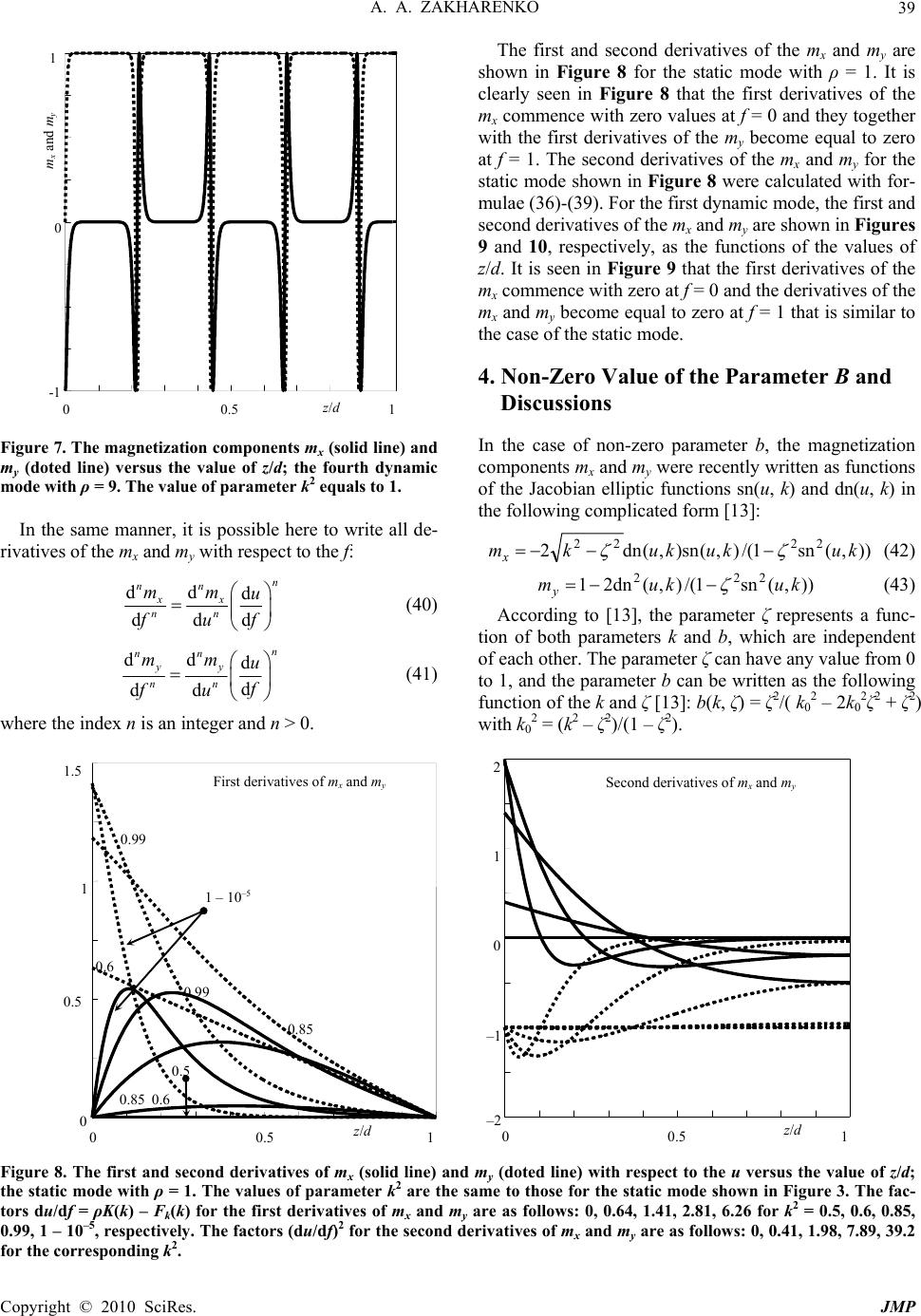

A. A. ZAKHARENKO 39
00.51
z
/
d
-1
0
1
m
x
and m
y
Figure 7. The magnetization components mx (solid line) and
my (doted line) versus the value of z/d; the fourth dynamic
mode with ρ = 9. The value of parameter k2 equals to 1.
In the same manner, it is possible here to write all de-
rivatives of the mx and my with respect to the f:
dd
d
d dd
n
nn
xx
nn
mm
u
f fu



(40)
dd
d
d dd
n
nn
yy
nn
mm
u
f fu



(41)
where the index n is an integer and n > 0.
The first and second derivatives of the mx and my are
shown in Figure 8 for the static mode with ρ = 1. It is
clearly seen in Figure 8 that the first derivatives of the
mx commence with zero values at f = 0 and they together
with the first derivatives of the my become equal to zero
at f = 1. The second derivatives of the mx and my for the
static mode shown in Figure 8 were calculated with for-
mulae (36)-(39). For the first dynamic mode, the first and
second derivatives of the mx and my are shown in Figures
9 and 10, respectively, as the functions of the values of
z/d. It is seen in Figure 9 that the first derivatives of the
mx commence with zero at f = 0 and the derivatives of the
mx and my become equal to zero at f = 1 that is similar to
the case of the static mode.
4. Non-Zero Value of the Parameter B and
Discussions
In the case of non-zero parameter b, the magnetization
components mx and my were recently written as functions
of the Jacobian elliptic functions sn(u, k) and dn(u, k) in
the following complicated form [13]:
)),(sn1/(),(sn),(dn2 2222 kukukukmx   (42)
)),(sn1/(),(dn21 222 kukum y   (43)
According to [13], the parameter ζ represents a func-
tion of both parameters k and b, which are independent
of each other. The parameter ζ can have any value from 0
to 1, and the parameter b can be written as the following
function of the k and ζ [13]: b(k, ζ) = ζ2/( k0
2 – 2k0 2ζ2 + ζ2)
with k0
2 = (k2 – ζ2)/(1 – ζ2).
First derivatives of m
x
and m
y
00.51
0
.5
1
1.5
0
z
/d
0.5
1 – 10
–5
0.85
0.99
0.6
0.85
0.99
0.6
00.51
–
2
–
1
0
1
2
z
/d
Second derivatives of m
x
and m
y
Figure 8. The first and second derivatives of mx (solid line) and my (doted line) with respect to the u versus the value of z/d;
the static mode with ρ = 1. The values of parameter k2 are the same to those for the static mode shown in Figure 3. The fac-
tors du/df = ρK(k) – Fk(k) for the first derivatives of mx and my are as follows: 0, 0.64, 1.41, 2.81, 6.26 for k2 = 0.5, 0.6, 0.85,
0.99, 1 – 10–5, respectively. The factors (du/df)2 for the second derivatives of mx and my are as follows: 0, 0.41, 1.98, 7.89, 39.2
for the corresponding k2.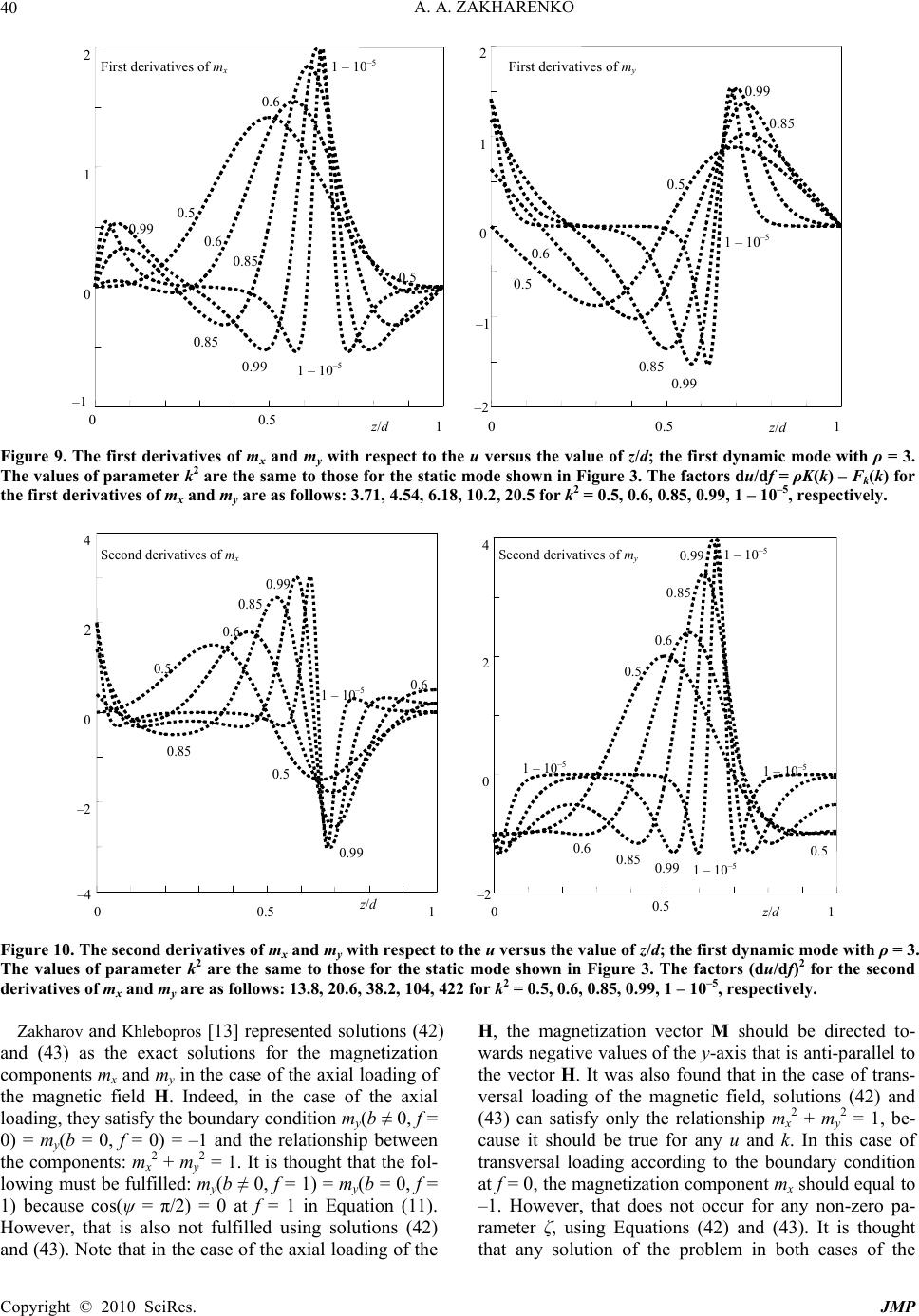

A. A. ZAKHARENKO 40
0 0.5 1
–
1
z
/d
0
1
2First derivatives of m
x
0.5
1
–
10
–5
0.85
0.99
0.6
0.85
0.99 0.6
0.5
1
–
10
–5
00.51
–
2
–
1
z
/d
0
1
2
0.5
1
–
10
–5
0.85
0.99
0.85
0.99
0.6
0.5
First derivatives of m
y
Figure 9. The first derivatives of mx and my with respect to the u versus the value of z/d; the first dynamic mode with ρ = 3.
The values of parameter k2 are the same to those for the static mode shown in Figure 3. The factors du/df = ρK(k) – Fk(k) for
the first derivatives of mx and my are as follows: 3.71, 4.54, 6.18, 10.2, 20.5 for k2 = 0.5, 0.6, 0.85, 0.99, 1 – 10–5, respectively.
0 0.5 1
–
4 z/d
–
2
0
2
4
0.5
1
–
10
–5
0.85
0.99
0.6
0.85
0.99
0.6
0.5
Second derivatives of m
x
00.5 1
–
2
z/d
0
2
4Second derivatives of m
y
0.5
1 – 10
–5
0.85
0.99
0.6
0.85
0.99
0.6
0.5
1
–
10
–5
1
–
10
–5
1
–
10
–5
Figure 10. The second derivatives of mx and my with respect to the u versus the value of z/d; the first dynamic mode with ρ = 3.
The values of parameter k2 are the same to those for the static mode shown in Figure 3. The factors (du/df)2 for the second
derivatives of mx and my are as follows: 13.8, 20.6, 38.2, 104, 422 for k2 = 0.5, 0.6, 0.85, 0.99, 1 – 10–5, respectively.
Zakharov and Khlebopros [13] represented solutions (42)
and (43) as the exact solutions for the magnetization
components mx and my in the case of the axial loading of
the magnetic field H. Indeed, in the case of the axial
loading, they satisfy the boundary condition my(b ≠ 0, f =
0) = my(b = 0, f = 0) = –1 and the relationship between
the components: mx
2 + my 2 = 1. It is thought that the fol-
lowing must be fulfilled: my(b ≠ 0, f = 1) = my(b = 0, f =
1) because cos(ψ = π/2) = 0 at f = 1 in Equation (11).
However, that is also not fulfilled using solutions (42)
and (43). Note that in the case of the axial loading of the
H, the magnetization vector M should be directed to-
wards negative values of the y-axis that is anti-parallel to
the vector H. It was also found that in the case of trans-
versal loading of the magnetic field, solutions (42) and
(43) can satisfy only the relationship mx
2 + my 2 = 1, be-
cause it should be true for any u and k. In this case of
transversal loading according to the boundary condition
at f = 0, the magnetization component mx should equal to
–1. However, that does not occur for any non-zero pa-
rameter ζ, using Equations (42) and (43). It is thought
that any solution of the problem in both cases of the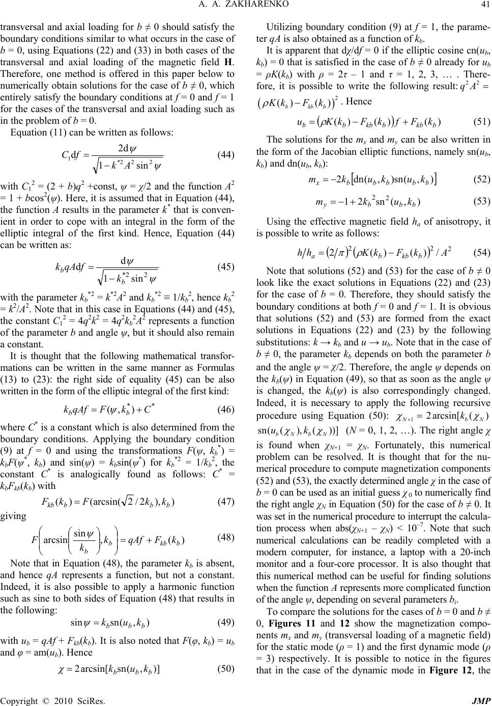

A. A. ZAKHARENKO 41
transversal and axial loading for b ≠ 0 should satisfy the
boundary conditions similar to what occurs in the case of
b = 0, using Equations (22) and (33) in both cases of the
transversal and axial loading of the magnetic field H.
Therefore, one method is offered in this paper below to
numerically obtain solutions for the case of b ≠ 0, which
entirely satisfy the boundary conditions at f = 0 and f = 1
for the cases of the transversal and axial loading such as
in the problem of b = 0.
Equation (11) can be written as follows:


222*
1sin1
2d
d
Ak
fC   (44)
with C1
2 = (2 + b)q2 +const, ψ = χ/2 and the function A2
= 1 + bcos2(ψ). Here, it is assumed that in Equation (44),
the function A results in the parameter k* that is conven-
ient in order to cope with an integral in the form of the
elliptic integral of the first kind. Hence, Equation (44)
can be written as:


22* sin1
d
d
b
b
k
fqAk   (45)
with the parameter kb
*2 = k*2A2 and kb *2 ≡ 1/kb 2, hence kb 2
= k2/A2. Note that in this case in Equations (44) and (45),
the constant C1
2 = 4q2k2 = 4q2kb 2A2 represents a function
of the parameter b and angle ψ, but it should also remain
a constant.
It is thought that the following mathematical transfor-
mations can be written in the same manner as Formulas
(13) to (23): the right side of equality (45) can be also
written in the form of the elliptic integral of the first kind:
** ),( CkFqAfk bb 
 (46)
where C* is a constant which is also determined from the
boundary conditions. Applying the boundary condition
(9) at f = 0 and using the transformations F(ψ, kb
*) =
kbF(ψ*, kb) and sin(ψ) = kbsin(ψ*) for kb
*2 = 1/kb 2, the
constant C* is analogically found as follows: C* =
kbFkb(kb) with
)),2/2(arcsin()( bbbkb kkFkF  (47)
giving
)(,
sin
arcsin bkbb
b
kFqAfk
k
F

















(48)
Note that in Equation (48), the parameter kb is absent,
and hence qA represents a function, but not a constant.
Indeed, it is also possible to apply a harmonic function
such as sine to both sides of Equation (48) that results in
the following:
),(snsin bbb kuk

(49)
with ub = qAf + Fkb(kb). It is also noted that F(φ, kb) = ub
and φ = am(ub). Hence
)],(snarcsin[2 bbb kuk

(50)
Utilizing boundary condition (9) at f = 1, the parame-
ter qA is also obtained as a function of kb.
It is apparent that dχ/df = 0 if the elliptic cosine cn(ub,
kb) = 0 that is satisfied in the case of b ≠ 0 already for ub
= ρK(kb) with ρ = 2τ – 1 and τ = 1, 2, 3, … . There-
fore, it is possible to write the following result:22
qA



2
() ()
bkbb
KkF k  . Hence

 )()()( bkbbkbbb kFfkFkKu 



(51)
The solutions for the mx and my can be also written in
the form of the Jacobian elliptic functions, namely sn(ub,
kb) and dn(ub, kb):

 ),(sn),(dn2 bbbbbxkukukm


(52)
),(sn21 2
2
bbby kukm (53)
Using the effective magnetic field ha of anisotropy, it
is possible to write as follows:




2
22 /)()(2 AkFkKhh bkbba 
 (54)
Note that solutions (52) and (53) for the case of b ≠ 0
look like the exact solutions in Equations (22) and (23)
for the case of b = 0. Therefore, they should satisfy the
boundary conditions at both f = 0 and f = 1. It is obvious
that solutions (52) and (53) are formed from the exact
solutions in Equations (22) and (23) by the following
substitutions: k → kb and u → ub. Note that in the case of
b ≠ 0, the parameter kb depends on both the parameter b
and the angle ψ = χ/2. Therefore, the angle ψ depends on
the kb(ψ) in Equation (49), so that as soon as the angle ψ
is changed, the kb(ψ) is also correspondingly changed.
Indeed, it is necessary to apply the following recursive
procedure using Equation (50): 1N

2arcsin[ () bN
k

sn(( ),( ))]
bN bN
uk

 (N = 0, 1, 2, …). The right angle χ
is found when χN+1 = χN. Fortunately, this numerical
problem can be resolved. It is thought that for the nu-
merical procedure to compute magnetization components
(52) and (53), the exactly determined angle χ in the case of
b = 0 can be used as an initial guess χ 0 to numerically find
the right angle χN in Equation (50) for the case of b ≠ 0. It
was set in the numerical procedure to interrupt the calcula-
tion process when abs(χN+1 – χN) < 10–7. Note that such
numerical calculations can be readily completed with a
modern computer, for instance, a laptop with a 20-inch
monitor and a four-core processor. It is also thought that
this numerical method can be useful for finding solutions
when the function A represents more complicated function
of the angle ψ, depending on several parameters bi.
To compare the solutions for the cases of b = 0 and b ≠
0, Figures 11 and 12 show the magnetization compo-
nents mx and my (transversal loading of a magnetic field)
for the static mode (ρ = 1) and the first dynamic mode (ρ
= 3) respectively. It is possible to notice in the figures
that in the case of the dynamic mode in Figure 12, the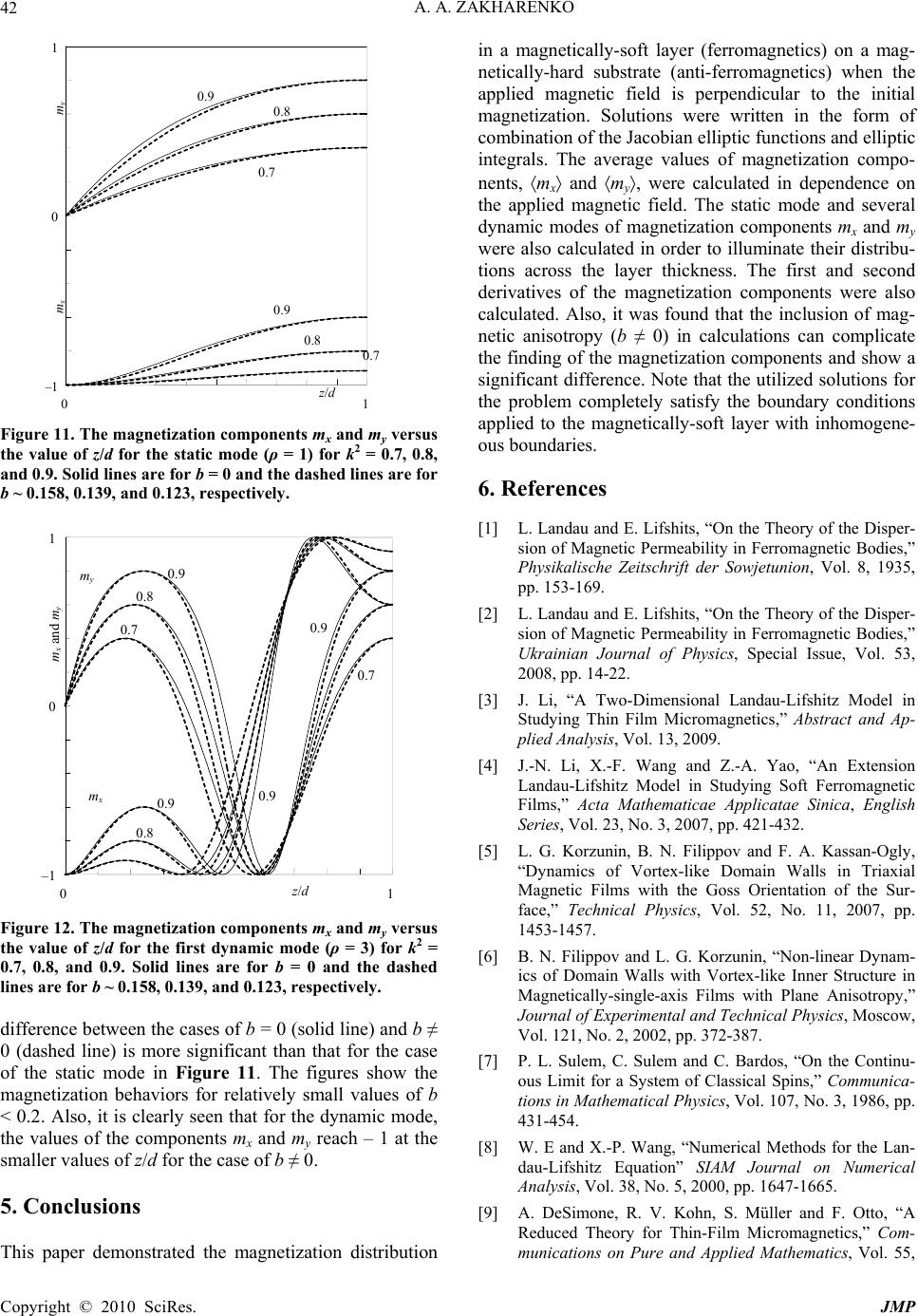

A. A. ZAKHARENKO 42
z
/d
m
x
m
y
0.8
0.7
0.9
0.9
0.8
0.7
01
–
1
0
1
Figure 11. The magnetization components mx and my versus
the value of z/d for the static mode (ρ = 1) for k2 = 0.7, 0.8,
and 0.9. Solid lines are for b = 0 and the dashed lines are for
b ~ 0.158, 0.139, and 0.123, respectively.
0 1
–
1
0
1
0.7
m
x
and m
y
0.8
0.7
0.9
0.8
0.9
0.9
0.9
m
x
m
y
z
/
d
Figure 12. The magnetization components mx and my versus
the value of z/d for the first dynamic mode (ρ = 3) for k2 =
0.7, 0.8, and 0.9. Solid lines are for b = 0 and the dashed
lines are for b ~ 0.158, 0.139, and 0.123, respectively.
difference between the cases of b = 0 (solid line) and b ≠
0 (dashed line) is more significant than that for the case
of the static mode in Figure 11. The figures show the
magnetization behaviors for relatively small values of b
< 0.2. Also, it is clearly seen that for the dynamic mode,
the values of the components mx and my reach – 1 at the
smaller values of z/d for the case of b ≠ 0.
5. Conclusions
This paper demonstrated the magnetization distribution
in a magnetically-soft layer (ferromagnetics) on a mag-
netically-hard substrate (anti-ferromagnetics) when the
applied magnetic field is perpendicular to the initial
magnetization. Solutions were written in the form of
combination of the Jacobian elliptic functions and elliptic
integrals. The average values of magnetization compo-
nents, mx and my, were calculated in dependence on
the applied magnetic field. The static mode and several
dynamic modes of magnetization components mx and my
were also calculated in order to illuminate their distribu-
tions across the layer thickness. The first and second
derivatives of the magnetization components were also
calculated. Also, it was found that the inclusion of mag-
netic anisotropy (b ≠ 0) in calculations can complicate
the finding of the magnetization components and show a
significant difference. Note that the utilized solutions for
the problem completely satisfy the boundary conditions
applied to the magnetically-soft layer with inhomogene-
ous boundaries.
6. References
[1] L. Landau and E. Lifshits, “On the Theory of the Disper-
sion of Magnetic Permeability in Ferromagnetic Bodies,”
Physikalische Zeitschrift der Sowjetunion, Vol. 8, 1935,
pp. 153-169.
[2] L. Landau and E. Lifshits, “On the Theory of the Disper-
sion of Magnetic Permeability in Ferromagnetic Bodies,”
Ukrainian Journal of Physics, Special Issue, Vol. 53,
2008, pp. 14-22.
[3] J. Li, “A Two-Dimensional Landau-Lifshitz Model in
Studying Thin Film Micromagnetics,” Abstract and Ap-
plied Analysis, Vol. 13, 2009.
[4] J.-N. Li, X.-F. Wang and Z.-A. Yao, “An Extension
Landau-Lifshitz Model in Studying Soft Ferromagnetic
Films,” Acta Mathematicae Applicatae Sinica, English
Series, Vol. 23, No. 3, 2007, pp. 421-432.
[5] L. G. Korzunin, B. N. Filippov and F. A. Kassan-Ogly,
“Dynamics of Vortex-like Domain Walls in Triaxial
Magnetic Films with the Goss Orientation of the Sur-
face,” Technical Physics, Vol. 52, No. 11, 2007, pp.
1453-1457.
[6] B. N. Filippov and L. G. Korzunin, “Non-linear Dynam-
ics of Domain Walls with Vortex-like Inner Structure in
Magnetically-single-axis Films with Plane Anisotropy,”
Journal of Experimental and Technical Physics, Moscow,
Vol. 121, No. 2, 2002, pp. 372-387.
[7] P. L. Sulem, C. Sulem and C. Bardos, “On the Continu-
ous Limit for a System of Classical Spins,” Communica-
tions in Mathematical Physics, Vol. 107, No. 3, 1986, pp.
431-454.
[8] W. E and X.-P. Wang, “Numerical Methods for the Lan-
dau-Lifshitz Equation” SIAM Journal on Numerical
Analysis, Vol. 38, No. 5, 2000, pp. 1647-1665.
[9] A. DeSimone, R. V. Kohn, S. Müller and F. Otto, “A
Reduced Theory for Thin-Film Micromagnetics,” Com-
munications on Pure and Applied Mathematics, Vol. 55,

A. A. ZAKHARENKO 43
No. 11, 2002, pp. 1408-1460.
[10] A. DeSimone, R. V. Kohn, S. Müller, F. Otto and R.
Schäfer, “Two-Dimensional Modelling of Soft Ferro-
magnetic Films,” Proceedings of the Royal Society of
London, Series A, Vol. 457, No. 2016, 2001, pp. 2983-
2991.
[11] A. Aharoni, E. H. Frei and S. Shtrikman, “Theoretical
Approach to the Asymmetrical Magnetization Curve,”
Journal of Applied Physics, Vol. 30, No. 12, 1959, pp.
1956-1961.
[12] N. M. Salansky and M. S. Eruchimov, “The Peculiarities
of Spin-Wave Resonance in Films with Ferro-Antiferro-
magnetic Interaction,” Thin Solid Films, Vol. 6, No. 2,
1970, pp. 129-140.
[13] Y. V. Zakharov and E. A. Khlebopros, “Magnetization
Curves and Frequencies of Magnetic Resonance in Films
with Domain Structures on Anti-Ferromagnetic Substrate,”
Solid State Physics, Moscow, Vol. 22, No. 12, 1980, pp.
3651-3657.
[14] H. Bateman and A. Erd´elyi, “Higher Transcendental
Functions,” McGraw-Hill, New York, Vol. 3, 1955.
[15] M. Abramowitz and I. A. Stegun, Eds., “Handbook of
Mathematical Functions with Formulas,” Graphs and
Mathematical Tables, National Bureau of Standards in
Applied Mathematics, Washington, 1964, p. 1058.
[16] L. Collatz, “Eigenvalue Problems with Engineering Ap-
plications,” Fizmatgiz, Moscow, 1968.
[17] Y. V. Zakharov, “Static and Dynamic Instability of a
Ferromagnetic Layer under Magnetic Reversal,” Doklady
of Russian Academy of Science, Vol. 344, No. 3, 1995, pp.
328-332.
[18] M. A. Lavrent’ev and A. Y. Ishlinskii, “Dynamic Buck-
ling Modes of Elastic Systems,” Doklady Akademii Nauk
USSR (Moscow), Vol. 64, No. 6, 1949, pp. 779-782.
[19] Y. V. Zakharov and A. A. Zakharenko, “Dynamic Insta-
bility in the Nonlinear Problem of a Cantilever,” Compu-
tational Technologies, Vol. 4, No. 1, 1999, pp. 48-54.
[20] M. Johnson, “Bipolar Spin Switch,” Science, Vol. 260 No.
5106, 1993, pp. 320-323.
[21] D. J. Monsma, J. C. Lodder, T. J. A. Popma and B. Dieny,
“Perpendicular Hot Electron Spin-Valve Effect in a New
Magnetic Field Sensor: The Spin-Valve Transistor,” Phy-
sical Review Letters, Vol. 74, No. 26, 1995, pp. 5260-
5263.
[22] M. Johnson, “Spin Injector in Metal Films: The Bipolar
Spin Transistor,” Materials Science and Engineering B,
Vol. 31, 1995, pp. 199-205.
[23] V. Y. Shur and E. L. Rumyantsev, “Kinetics of Ferro-
electric Domain Structure during Switching: Theory and
Experiment,” Ferroelectrics, Vol. 151, 1994, pp. 171-189.