Journal of Modern Physics
Vol. 2 No. 8 (2011) , Article ID: 7123 , 10 pages DOI:10.4236/jmp.2011.28106
Coupling Interactions and Trapped Effects for a Triple-Well Potential
Department of Physics, Faculty of Sciences, Gazi University, Ankara, Turkey
E-mail: msimsek@gazi.edu.tr
Received March 24, 2011; revised May 6, 2011; accepted May 20, 2011
Keywords: Perturbation Method, Triple-Well Potential, Duffing Equation, Weak and Strong Couplings.
ABSTRACT
Weak and strong coupling interactions and trapped effects have always played a significant role in understanding physical and chemical properties of materials. Triple-well anharmonic potential may be modeled for interpretation of energy spectra from the nuclear to macro molecular systems, and also crystalline systems. Exact periods of a trapped particle in each well of the potential are explicitly derived. For the extended Duffing system, it is predicted that infinite series of both frequency and spatial trajectory approach to exact results in the limit of weak-coupling cases (g→0).
1. Introduction
The physics of nonlinear systems is one of the important research interests in both quantum and classical mechanics, and its oscillatory representation [1-7] occupies special place for dynamical systems. There are different kinds of nonlinear oscillator problems that arise in the study of dynamical systems. In that, the extension of well-known nonlinear pendulum theory to the one dimensional oscillator model has been widely used to simulate classical and quantum systems (see some of references [1-17]).
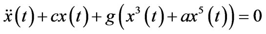
Nonlinear oscillatory systems are widely used tools for the modeling of atomic, molecular and crystalline systems [12-23]. Although overall reliability of the quantum and classical interpretations is controversial, the simple theoretical correspondence and appropriate calculations make them popular, among the theoretically physicists and chemists [19-25]. Now, let us consider a second order one dimensional anharmonic oscillator equation,
 (1)
(1)
with the arbitrary parameters of c, g and a. Note that if the parameters in the equation are chosen as c = w02, g = –1/6 w02 and a = –1/20, it turns to fifth order non-linear equation of elementary (1+1) dimensionally pendulum, and also to the Duffing equation [26-28] for a = 0. However, using the perturbation approximations [21], a model of nonlinear problem, other words the extended Duffing equation, reduces to approximately solvable case. So, we called it here after the extended Duffing oscillator.
It is important that the range of applicability of this equation is fairly wide than that of Duffing oscillator, and in particular, it includes extra free parameter (a). Other words, the arbitrary parameters (i.e., g and a) stand for the perturbation parameter and coupling constants for weak-coupling systems, respectively. It may be modeled for coherent tunneling via adiabatic passage in a triplewell system and coherent transport of electrons between quantum dots or atoms in micro-magnetic traps [18]. Generally, for weak-coupling systems, anharmonic terms can be treated as a perturbation, that well-known first detailed example is quartic anharmonic potential by Bender and Wu [24, 25]. By our assumptions, in order to parallel analysis, this new nonlinear equation may be called Duffing+ax5 equation.
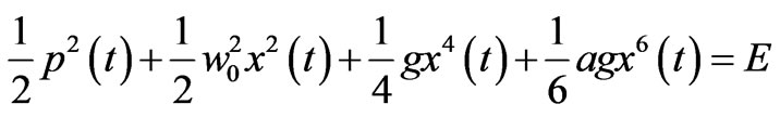
Let us integrate the dynamical system in Equation (1) with respect to time,
 ,
,
 (2)
(2)
where the integral constant E (Energy) can be imposed in terms of the potential parameters. By using the initial conditions for frequency (w0) and location (x0) at t = 0, and also for the parameters a and g, it can be settled as,

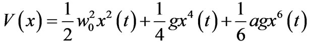
So, the reducible potential in Equation (2) can be written as,
 (3)
(3)
which has different shapes, as a modeling of systems, for given potential parameters w0, a and g (see Figure 1). Note that, if one wants to get the special shapes of the potential, such as one and two or three wells, the restrictions must be constructed among the parameters as in Table 1, which shows the possible range of the potential parameters for triple-well behavior.
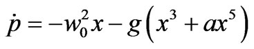
On the other hand, for given initial energy (E) and initial parameters, dynamical equation of the system in Equation (2) can be written as,
 ,
,
 (4)
(4)
For chosen g and a parameters, which they are generating three-well and one-well potentials, phase portraits are shown in Figures 2 (a) and (b), respectively. It is seen that the closed orbits are for bonded cases in the trajectories, are correspond different potential shapes. However, both of bounded (closed orbits) and unbounded cases (open orbits) can be situated, i.e., all initial conditions could not lead to the stable equilibrium points and closed orbits. Other words, the image of a periodic solution in the phase portrait is a closed trajectory that is usually called periodic orbit also. Therefore, instead of trying to
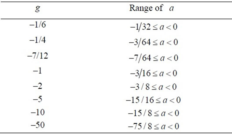
Table 1. The range of the parameter  for given some g values of triple-well potentials in the interval
solve the equation for all phase paths, we would like to find the periodic solutions as
 (5)
(5)
for the bonded cases, with the initial conditions,
 ,
, (6)
(6)
By our initial assumptions, we apply the LindstedtPoincaré perturbation method [26-28] to the non-linear Duffing + ax5 oscillatory system, in following section (Section 2). In Section 3, we derive the exact quarter periods expressions for a particle in the triple-well potential. Hence, we calculate the weak and strong interaction
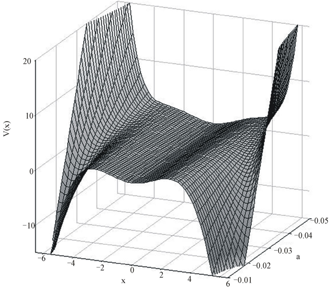
Figure 1. The shapes of triple–well (sextic oscillator) potential versus anharmonicity parameters a, and x. The other anharmonicity parameter is fixed (g = –1/6) to treat pendulum problem.
 (a)
(a)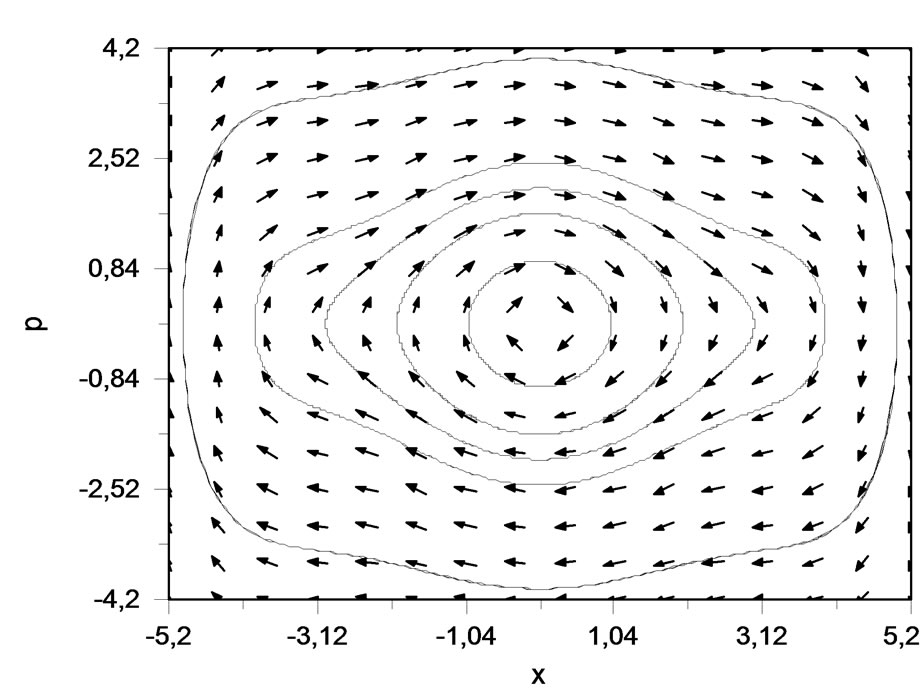 (b)
(b)
Figure 2. The phase portraits of sextic anharmonic oscillator potential with fixed g = –1/6 and different values of anharmonicity parameter a; a) for tree-finite gap cases, a = –3/100; and b) for one-finite gap cases, a = –5/100. The values of the parameters chosen as the corresponding coefficients of the Taylor expansion of sin(θ).
limit cases for the purposed system in Sec.4. Finally, the paper ends with discussion section Sec.5.
2. Weak-Coupling Interactions
Classical Lindstedt-Poincaré approach [26-28], it’s modified version [23, 29-30] and also linear delta expansion method [31] are powerful methods for generating periodic perturbation series of the non-linear anharmonic oscillatory systems. We now consider rescale time according to
 (7)
(7)
then, Equation (1) can be written as
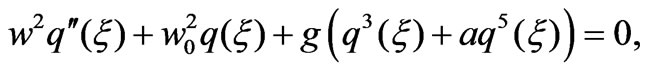 (8)
(8)
with the initial conditions,  , where, the prime denotes differentiation with respect to new time variable, ξ. Thus, the periodicity is
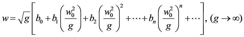
  for new variables. The fact that periodic solutions of equations can be expressed as an infinite series [23] for small coupling parameter (
 ),
),
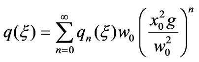 (9)
(9)
and also, frequency w can be expanded as
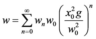 (10)
(10)
Then, substituting series of w and q(ξ) in Equation (8) and comparing the coefficients of the same power of the perturbation parameter g, it can be obtained a recursive set of simple ordinary differential equations:
 (11)
(11)
where
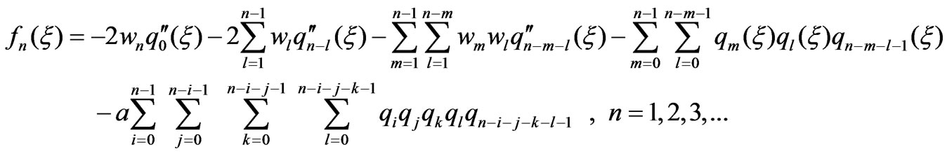 (12)
(12)
without impairing the generality, we can impose initial values: w0 = 1 and x0 = 1. The initial trajectory could be chosen as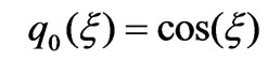 . Otherwise,
  functions can be expanded to a Fourier series
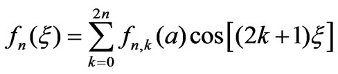 (13)
(13)
with starting coefficients as fn,0 = 0. Note that choosing of this initial value, the secular terms in the solutions of Equation (11) are vanish. On the other hand, we can write
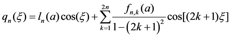 (14)
(14)
where
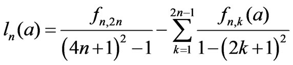 (15)
(15)
Note that, these general expressions can be predicted analytically using simple algebra. Substituting general definitions (12-13) in differential Equation (11), we find the corresponding series for and
and  (Equations (9) and (10)),
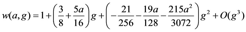 (16)
(16)

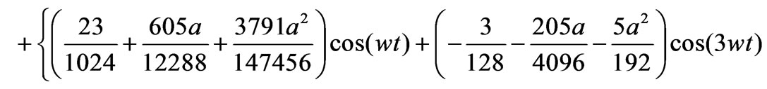
 (17)
(17)
It is note that, these infinity series of w(a,g) approach the exact results in the limit g→0 for the weak-coupling systems and, the series of trajectory x(w,a,g;t) coincide with the fourth-order Runge-Kutta method results. On the other hand, it is seen that when a is choosed as zero, this formulation is reduced to solution of well-known Duffing oscillator [9-11,23,26-28]. However, fn,k(a) and ln(a) functions are listed in Tables 2 and 3, respectively.
3. Exact Solutions of a Particle in the Triple-Well Potential
Classically, it is simple to combine time and space variables under certain conditions. Substituting p (from Equation (4)), it can be integrated over a quarter period. Thus, we obtain exact quarter period for a particle in the triple-well potential as
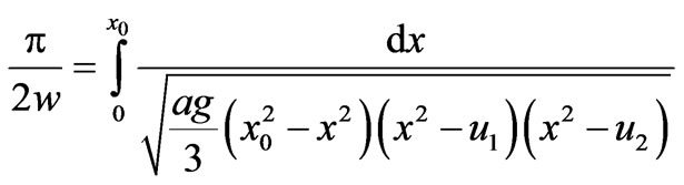 (18)
(18)
where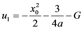 , and
, and
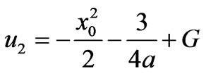 with
with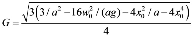 .
.
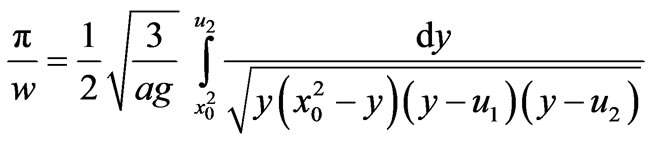
Changing the variable x2 = y, period integral turns to
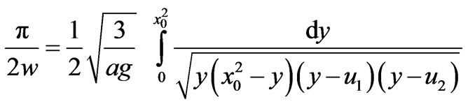 (19)
(19)
and help of integral tables in Ref.[32] (equation number is 3.147), we can calculate the last integral. For given possible energies or initial conditions, a matter of practical importance is to determine the classical period of trapped particle. Now, let us suppose the potential have three well (see Figure 1). and a particle has been trapped one of the wells. It is note that the use of different values
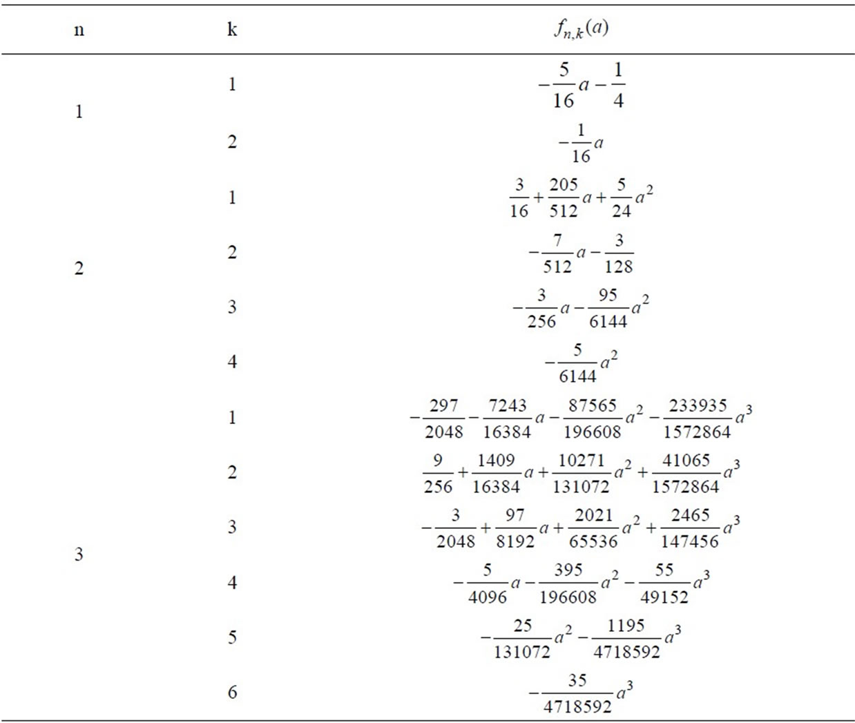
Table 2. The coefficients of inhomogeneous oscillatory equations,  , of weak coupling cases
  in Equation (13). Coefficients were computed using Equation (13).
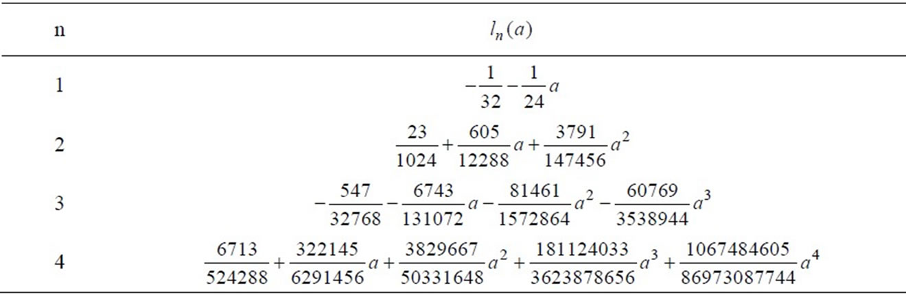
Table 3. The coefficients of the solutions of weak coupling cases  in Equation (14), which were calculated using Equation (15). Coefficients depend on coupling parameter a.
of potential parameters leads to different varieties of potential shapes and equilibrium conditions. Therefore, having defined equilibrium points, our task now is to find period of trapped particle in one of potential wells:
1) At middle well: choosing the parameters as, 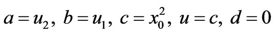 , and then using the equation (3.147.2) in Ref. [32],
 (20)
(20)
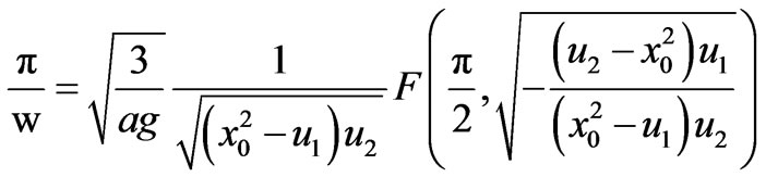
we can find the exact quarter period as
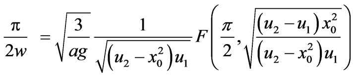 (21)
(21)
where 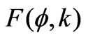 is elliptic integral of the first kind [32]
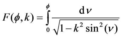 (22)
(22)
2) At right (or left) well: there are two different cases. If the particle has positive energy, we set the parameters as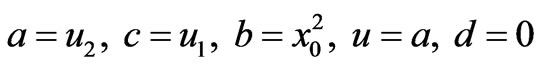 , and then, we use the equation (3.147.6) in Ref. [32],
 (23)
(23)
Thus, we can find exact half period of particle with positive energy as
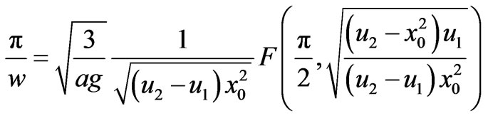 (24)
(24)
On the other hand, if the particle has negative energy and in right (or left) well, we set the parameters as: , and then using equation (3.147.6) in Ref.[32],
 (25)
(25)
we can find the exact half period as
 (26)
(26)
It is note that, if we expand Equation (21) for limit (g→0), as expected for weak coupling cases, there is an excellent agreement between expansion and Equation (16), i.e., they are the same.
4. Strong-Coupling Limit
Let us rewrite Equation (21), for middle range, as
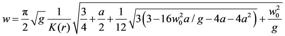 (27)
(27)
where K(r)=F(p/2, r) is elliptic K function, (8.112.1) in Ref.[32],. The new variable is 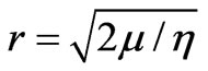 with
with
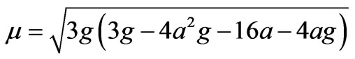 ,
,
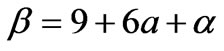
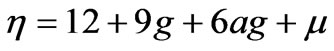 respectively . Our purpose is to find the series expansion of the periods in large asymptotic limit, g→∞. Hence, we can write frequency series as,
 (28)
(28)
where first three coefficients are
 (29)
(29)
and,
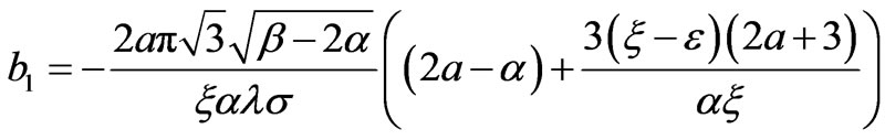 (30)
(30)

with the abbreviations
 ,
,  ,
,  ,
,
 ,
,
 ,
, 
 ,
,  ,
, ,
,  ,
,
 respectively.
In order to compare, we figure out the weak-coupling and strong-coupling expansions together with the exact result in Figure 3. It can be indicated that the curve of exact result is appearing as a ‘cut line’ between last term of the expansions odd and even order for two different classes of interactions. In the other words, if the order of last term of expansion is even (odd) then, corresponding curve lies below (above) the curve of exact results. Note that the plot of extended Duffing systems is similar to that of the Duffing systems (see Figure 1 in Ref. [23]). In Figure 4, we plot of weak-coupling perturbation series (10) versus to the coupling parameter a for fixed g = –1/6, where corresponding perturbation orders are marked in label (1 - 11). It should also be noted that, as expected for weak-coupling cases, the convergence rate increases while value of a decreases (see Figure 4).
In addition to the Duffing systems, a more general situation has been investigated for the Duffing and Duffing+ax5 dynamical systems. On the other hand, we also solve the equation by numerical Runge-Kutta (RK) method that, the solutions coincide with LP profiles only in small absolute value of parameter g (|g|<1). The results are shown in Figure 5, where we plot spatial profile of oscillator versus time. These results are interesting not only in the convergence of both dynamical properties but also in the context of realistic physical systems. It is shown that period of system increases, while the absolute value of parameter g decreases.
5. Conclusions
We have shown that dynamical solutions of the extended Duffing oscillator, the corresponding to the family of quantum triple-well potentials can be closely approximated by choosing appropriate potential parameters. The basic advantages of the approach are due to its specific properties of quantum triple-well oscillator potential. We can say that our algorithm is more flexible for other polynomial potentials, and also reproduces infinite perturbation series for the trajectories and the frequencies of a trapped particle within limit of weak and strong coupling interactions. Of course, weak and strong coupling interactions and the trapped effects are important inmany fields of physics such as particle physics, atomic, molecular and macromolecular systems. It should be remarked that, there is a good agreement between the
Figure 3. The plot of exact result is versus coupling parameter g for middle range of potential (solid curve). For the parameter, a = –3/100, the truncated perturbation expansions of weak-coupling cases (dashed curves) are labeled with  and the strong coupling cases (dotted curves) with
 .
.
Figure 4. The plot of weak-coupling perturbation series (10) versus parameter a for middle range (for fixed g = –1/6). The numbers at the figure indicate that the order of perturbation series.
Figure 5. Numerically and approximately (with perturbation theory) calculated profiles of trajectory,  , for different values of the perturbation parameter g. In the figure, the value of the parameter a = –3/100, and n denotes the order of perturbation.
results of the Lindstedt-Poincaré perturbation method and our analytic results for weak coupling cases.
REFERENCES
- J. H. He, “An Elementary Introduction to Recently Developed Asymptotic Methods and Nanomechanics in Textile Engineering,” International Journal of Modern Physics B, Vol. 22, No. 21, 2008, pp. 3487-3578. doi:10.1142/S0217979208048668
- F. M. Fernandez and R. H. Tipping, “Accurate Calculation of Vibrational Resonances by Perturbation Theory,” Journal of Molecular Structure (Theochem), Vol. 488, No. 1-3, 1999, pp. 157-161. doi:10.1016/S0166-1280(98)00622-8
- F. J. Gomez and J. Sesma, “Bound States and “Resonances” in Quantum Anharmonic Oscillators,” Physics Letters A, Vol. 270, No. 1-2, 2000, pp. 20-26. doi:10.1016/S0375-9601(00)00290-5
- A. Pathak and S. Mandal, “Classical and Quantum Oscillators of Quartic Anharmonicities: Second-Order Solution,” Physics Letters A, Vol. 286, No. 4, 2001, pp. 261-276. doi:10.1016/S0375-9601(01)00401-7
- A. Pathak and S. Mandal, “Classical and Quantum Oscillators of Sextic and Octic Anharmonicities,” Physics Letters A, Vol. 298, No. 4, 2002, pp. 259-270. doi:10.1016/S0375-9601(02)00500-5
- Y. Meurice, “Arbitrarily Accurate Eigenvalues for One-Dimensional Polynomial Potentials,” Journal of Physics A: Mathematical and General, Vol. 35, No. 41, 2002, pp. 8831-8846. doi:10.1088/0305-4470/35/41/314
- I. A. Ivanov, “Transformation of the Asymptotic Perturbation Expansion for the Anharmonic Oscillator into a Convergent Expansion,” Physics Letters A, Vol. 322, No. 3-4, 2004, pp. 194-204. doi:10.1016/j.physleta.2004.01.014
- H. K. Khalil, “Nonlinear Systems,” Maxwell Macmillan, Toronto, 1992.
- J. H. He, “Some New Approaches to Duffing Equation with Strongly and High Order Nonlinearity (II) Parametrized Perturbation Technique,” Communications in Nonlinear Science and Numerical Simulation, Vol. 4, No. 1, 1999, pp. 81-83. doi:10.1016/S1007-5704(99)90065-5
- J. Lin, “A New Approach to Duffing Equation with Strong and High Order Nonlinearity,” Communications in Nonlinear Science and Numerical Simulation, Vol. 4, No. 2, 1999, pp. 132-135. doi:10.1016/S1007-5704(99)90026-6
- J. H. He, “Variational Iteration Method—a Kind of Non-Linear Analytical Technique: Some Examples,” International Journal of Non-Linear Mechanics, Vol. 34, No. 4, 1999, pp. 699-708. doi:10.1016/S0020-7462(98)00048-1
- Y. Z. Chen, “Solution of the Duffing Equation by Using Target Function Method,” Journal of Sound and Vibration, Vol. 256, No. 3, 2002, pp. 573-578. doi:10.1006/jsvi.2001.4221
- A. R. Chouikha, “Series Solutions of Some Anharmonic Motion Equations,” Journal of Mathematical Analysis and Applications, Vol. 272, No. 1, 2002, pp. 79-88. doi:10.1016/S0022-247X(02)00134-8
- M. El-Kady and E. M. E. Elbarbary, “A Chebyshev Expansion Method for Solving Nonlinear Optimal Control Problems,” Applied Mathematics and Computation, Vol. 129, No. 2-3, 2002, pp. 171-182. doi:10.1016/S0096-3003(01)00104-7
- C. W. Lim and B. S. Wu, “A New Analytical Approach to the Duffing-Harmonic Oscillator,” Physics Letters A, Vol. 311, No. 4-5, 2003, pp. 365-373. doi:10.1016/S0375-9601(03)00513-9
- Y. Z. Chen, “Evaluation of Motion of the Duffing Equation from Its General Properties,” Journal of Sound and Vibration, Vol. 264, No. 2, 2003, pp. 491-497. doi:10.1016/S0022-460X(02)01495-5
- H. R. Marzban and M. Razzaghi, “Numerical Solution of the Controlled Duffing Oscillator by Hybrid Functions,” Applied Mathematics and Computation, Vol. 140, No. 2-3, 2003, pp. 179-190. doi:10.1016/S0096-3003(02)00112-1
- T. Opatrný and K. K. Das, “Conditions for Vanishing Central-Well Population in Triple-Well Adiabatic Transport,” Physics Letters A, Vol. 79, No. 1, 2009, p. 02113.
- V. B. Mandelzweig and F. Tabakin, “Quasilinearization Approach to Nonlinear Problems in Physics with Application to Nonlinear ODEs,” Computer Physics Communications, Vol. 141, No. 2, 2001, pp. 268-281. doi:10.1016/S0010-4655(01)00415-5
- J. I. Ramos, “Linearization Methods in Classical and Quantum Mechanics,” Computer Physics Communications, Vol. 153, No. 2, 2003, pp. 199-208. doi:10.1016/S0010-4655(03)00226-1
- J. L. Trueba, J. P. Baltanas and M. A. F. Sanjuan, “A generalized Perturbed Pendulum,” Chaos, Solitons & Fractals, Vol. 15, No. 5, 2003, pp. 911-924. doi:10.1016/S0960-0779(02)00210-2
- A. Post and W. Stuiver, “Modeling Non-Linear Oscillators: A New Approach,” International Journal of NonLinear Mechanics, Vol. 39, No. 6, 2004, pp. 897-908. doi:10.1016/S0020-7462(03)00073-8
- A. Pelster, H. Kleinert and M. Schanz, “High-Order Variational Calculation for the Frequency of Time-Periodic Solutions,” Physical Review E, Vol. 67, No. 1, 2003, p. 016604. doi:10.1103/PhysRevE.67.016604
- C. M. Bender and T. T. Wu, “Analytic Structure of Energy Levels in a Field-Theory Model,” Physical Review Letters, Vol. 21, No. 6, 1968, pp. 406-409. doi:10.1103/PhysRevLett.21.406
- C. M. Bender and T. T. Wu, “Anharmonic Oscillator,” Physical Review, Vol. 184, No. 5, 1969, pp. 1231-1260. doi:10.1103/PhysRev.184.1231
- J. J. Stoker, “Nonlinear Vibrations,” Interscience, New York, 1950.
- N. Minorsky, “Nonlinear Oscillation,” Van Nostrand, Princeton, 1962.
- A. H. Nayfeh, “Introduction to Perturbation Techniques,” John Wiley, New York, 1981.
- J. H. He, “Modified Lindstedt–Poincare Methods for Some Strongly Non-Linear Oscillations: Part I: Expansion of a Constant,” International Journal of Non-Linear Mechanics, Vol. 37, No. 2, 2002, pp. 309-314. doi:10.1016/S0020-7462(00)00116-5
- J. H. He, “Modified Lindstedt–Poincare Methods for Some Strongly Non-Linear Oscillations: Part II: A New Transformation,” International Journal of Non-Linear Mechanics, Vol. 37, No. 2, 2002, pp. 315-320. doi:10.1016/S0020-7462(00)00117-7
- P. Amore and A. Aranda, “Presenting a New Method for the Solution of Nonlinear Problems,” Physics Letters A, Vol. 316, No. 3-4, 2003, pp. 218-225. doi:10.1016/j.physleta.2003.08.001
- L. S. Gradshteyn and L. M. Rhyzik, “Table of Integrals, Series and Products,” Academic Press, New York, 1980.