Received 6 October 2015; accepted 27 November 2015; published 30 November 2015

ABSTRACT

In this paper, we used two different algorithms to solve some partial differential equations, where these equations originated from the well-known two parameters of logistic distributions. The first method was the classical one that involved solving a triply of partial differential equations. The second approach was the well-known Darboux Theory. We found that the geodesic equations are a pair of isotropic curves or minimal curves. As expected, the two methods reached the same result.

Keywords:

Darboux Theory, Differential Geometry, Geodesic Equation, Isotropic Curves, Logistic Distribution, Minimal Curves, Partial Differential Equation

1. Introduction

In general, we confine ourselves to real geometric objects, and consequently, to real functions of real variables. Nevertheless, it is sometimes advantageous to introduce complex variables as a tool for the investigation of real surfaces. This means we should regard the real Euclidean space as being embedded in a complex Euclidean space. A curve is said to be an isotropic curve or minimal curve if the length of the arc between any two different points of the curve is zero.

Hence, a curve is isotropic if and only if. This means the isotropic curve cannot have real solutions, but has two conjugate complex ones. Actually, the isotropic curves are always complex curves. In this paper, we used two different algorithms and found that the geodesic equation of Logistic distribution is a pair of complex curves or imaginary curves. In the next section, we summarized the fundamental tensor for later use. In Section 3, we use two different algorithms to derive the geodesic equation of logistic distributions. In Section 4, we give a more detailed explanation of how the fundamental tensor can be derived. An interesting work would be to compare our mathematical models with Mitchell, A.F.S. [1] [2] predictive distance model that is based on the statistical Beyesian Theory. There are lots of literatures related to distributional distance problem. For example, Kass R.E., Vos P.W. [3] and Amari S-I [4] have systematically introduced these concepts while Jensen U. [5] has applied this idea to quantitative economics.

2. List the Fundamental Tensor

The probability density function for the logistic distribution is given by

where v is the scale parameter, and u is the location parameter.

From above equation, we derive the metric tensor components for the logistic case as follows,

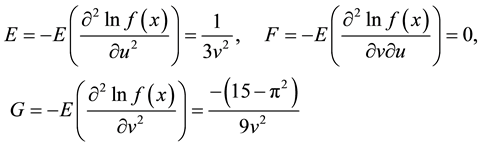
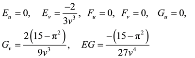
Using above results, we can easily find the required tensor metric

3. The Geodesic Equation

One method to find the geodesic equation of the logistic distribution is by solving a triply of partial differential equations given in the Appendix 1 (see Struik, D.J. or Grey, A [6] [7] ). We seek its solution in the following section.

To avoid confusing, we only index those formulas we will use them later and ignore the other.

(1)

(2)

And the distance function is given by

(3)

It needs only two out of the three equations above to find the logistic model of geodesic equation. We will choose the Equations (1) and (3). To simplify the notation, we let

(4)

Dividing the Equation (4) by p, and integrating on both sides with respect to p, we get

(5)

(6)

Inverse Equation (5) and solve for then square both side to get. Since e raise a constant power is still a constant. If we wish to get the same results as Darboux method then we just let constant, , equal constant. In other words, we choose constant.

After substituting (6) into (3), we can derive the following results

Integrating both sides, we find the geodesic equation

where A and B are arbitrary constants

Alternatively, we can find the geodesic equation of the logistic distribution by solving one partial differential equation. This idea originated from French mathematician Darboux’s theory. A detailed proof has been given in Chen [8] [9] . From section 2, we know that the coefficient of the first fundamental form of is given by,

To solve the partial differential equation above, we may use the separable variable method as follows.

The general solution of the geodesic equation is

where A and B are arbitrary constants. This result is the same as the previous one.

4. Deriving the Basic Tensor

The probability density function for the logistic distribution is given by

From the equation above, we derive the metric tensor components for the logistic case as follows,

The next step we need to find the moments of these partial derivatives. Some of these expectations are tricky and messy.

The first part of integral can easily check is zero since and use integral by part

While the second part is also zero, We can write the expectation as

The last expectation is messy and tricky.

To see the result of second part expectation,

Now, we check third part expectation,

Cite this paper

William W. S.Chen, (2015) On Finding Geodesic Equation of Two Parameters Logistic Distribution. Applied Mathematics,06,2169-2174. doi: 10.4236/am.2015.612189

References

Appendix 1

We list the six well known Christoffel Symbols as follows. For detail derivation see Struik [4] or Grey [5] .

In general, the solution of the geodesic equation depends upon a pair of partial differential equations as below.

Appendix 2

For detail derivation see reference [10] [11] (Appendix 2).

where is the Riemann zeta function defined by

And the well known fact that

References

- 1. Mitchell, A.F.S. (1992) Estimative and Predictive Distances. Test, 1, 105-121.
http://dx.doi.org/10.1007/BF02562666 - 2. Mitchell, A.F.S. and Krzanowski, W.J. (1985) The Mahalanobis Distance and Elliptic Distributions. Biometrika, 72, 464-467.
http://dx.doi.org/10.1093/biomet/72.2.464 - 3. Kass, R.E. and Vos, P.W. (1997) Geometrical Foundations of Asymptotic Inference. John Wiley & Sons, Inc.
http://dx.doi.org/10.1002/9781118165980 - 4. Amari, S.-I. (1990) Differential-Geometrical Methods in Statistics. Springer, New York.
- 5. Jensen, U. (1995) Review of “The Derivation and Calculation of Rao Distances with an Application to Portfolio Theory”. In: Maddala, P., Phillips, G.S. and Srinivasan, T., Eds., Advances in Econometrics and Quantitative Economics: Essays in Honor of C.R. Rao, Blackwell, Cambridge, 413-462.
- 6. Struik, D.J. (1961) Lectures on Classical Differential Geometry. 2nd Edition, Dover Publications, Inc.
- 7. Grey, A. (1993) Modern Differential Geometry of Curves and Surfaces. CRC Press, Inc., Boca Raton.
- 8. Chen, W.W.S. (2014) A Note on Finding Geodesic Equation of Two Parameters Gamma Distribution. Applied Mathematics, 5, 3511-3517. www.scirp.org/journal/am
http://dx.doi.org/10.4236/am.2014.521328 - 9. Chen, W.W.S. (2014) A Note on Finding Geodesic Equation of Two Parameter Weibull Distribution. Theoretical Mathematics & Applications, 4, 43-52.
- 10. Balakrishnan, N. and Nevzorov, V.B. (2003) A Primer on Statistical Distributions. John Wiley & Sons, Inc.
- 11. Gradshteyn, I.S., Ryzhik, I.M. and Jeffrey, A. (1994) Table of Integrals, Series, and Products. 5th Edition, Academic Press.