Received 26 November 2014; accepted 12 December 2014; published 19 January 2015

ABSTRACT

Invertibility is one of the desirable properties of moving average processes. This study derives consequences of the invertibility condition on the parameters of a moving average process of order three. The study also establishes the intervals for the first three autocorrelation coefficients of the moving average process of order three for the purpose of distinguishing between the process and any other process (linear or nonlinear) with similar autocorrelation structure. For an invertible moving average process of order three, the intervals obtained are, and.

Keywords:

Moving Average Process of Order Three, Characteristic Equation, Invertibility Condition, Autocorrelation Coefficient, Second Derivative Test

1. Introduction

Moving average processes (models) constitute a special class of linear time series models. A moving average process of order (process) is of the form:

(1.1)

where are real constants and, is a sequence of independent and identically distributed random variables with zero mean and constant variance. These processes have been widely used to model time series data from many fields [1] -[3] . The model in (1.1) is always stationary. Hence, a required condition for the use of the moving average process is that it is invertible. Let, then the model in (1.1) is invertible if the roots of the characteristic equation

(1.2)

lie outside the unit circle. The invertibility conditions of the first order and second order moving average models have been derived [4] [5] .

Ref. [6] used a moving average process of order three (MA (3) process) in his simulation study. Though, higher order moving average processes have been used to model time series data, not much has been said about the properties of their autocorrelation functions. This study focuses on the invertibility condition of an MA (3) process. Consideration is also given to the properties of its autocorrelation coefficients of an invertible moving average process of order three.

2. Consequence of Invertibility Condition on the Parameters of an MA (3) Process

For, the following moving average process of order 3 is obtained from (1.1):

(2.1)

The characteristic equation corresponding to (2.1) is given by

(2.2)

Dividing (2.2) by yields

(2.3)

It is important to know that (2.2) is a cubic equation. Detailed information on how to solve cubic equations can be found in [7] [8] among others. It has been a common tradition to consider the nature of the roots of a characteristic equation while determining the invertibility condition of a time series model [9] . As a cubic equation, (2.2) may have three distinct real roots, one real root and two complex roots, two real equal roots or three real equal roots. The nature of the roots of (2.2) is determined with the help of the discriminant [8]

(2.4)

where

(2.5)

and

(2.6)

If, (2.2) has the following distinct roots [7]

, (2.7)

, (2.8)

and

. (2.9)

where is measured in radians and.

When, (2.2) has only real root given by [1] as

(2.10)

The other roots are [8]

(2.11)

If, and, then and (2.2) has two equal roots. The roots of (2.2) in this case, are the same as (2.7), (2.8) and (2.9). For and, (2.2) has three real equal roots. Each of these roots is given by [8] as

(2.12)

For (2.1) to be invertible, the roots of (2.2) are all expected to lie outside the unit circle and. In the following theorem, the invertibility conditions of an MA (3) process are given subject to the condition that the corresponding characteristic equation has three real equal roots.

Theorem 1. If the characteristic equation has three real equal roots, then the moving average process of order three is invertible if

, and.

Proof

For invertibility, we expect each of the three real equal roots to lie outside the unit circle. Thus,

or

Solving the inequality, we obtain

For, we have

Since each of the roots lie outside the unit circle, the absolute value of their product must therefore be greater than one. Hence,

This completes the proof.

The invertibility region of a moving average of order three with equal roots of the characteristic Equation (2.2) is enclosed by triangle OAB in Figure 1.

3. Identification of Moving Average Process

Model identification is a crucial aspect of time series analysis. A common practice is to examine the structures of the autocorrelation function (ACF) and partial autocorrelation function (PACF) of a given time series. In this regard, a time series is said to follow a moving average process of order if its associated autocorrelation function cut off after lag and the corresponding partial autocorrelation function decays exponentially [10] . Authors using this method, believe that each process has unique ACF representation. However, the existence of similar autocorrelation structures between moving average process and pure diagonal bilinear time series process of the same order makes it difficult to identify a moving average process based on the pattern of its ACF. Furthermore, a careful look at the autocorrelation function of the square of a time series can help one determine if the series follows a moving average process. If the series can be generated by a moving average process, then its square follows a moving average process of the same order [11] [12] . The conditions under which we use the autocorrelation function to distinguish among processes behaving like moving average processes of order one and two have been determined by [13] [14] respectively. These conditions are all defined in terms of the extreme values of autocorrelation coefficients of the processes.

4. Intervals for Autocorrelation Coefficients of a Moving Average Process of Order Three

As stated in Section 3, knowledge of the extreme values of the autocorrelation coefficient of a moving average process of a particular order can enable us ensure proper identification of the process. It has been observed that for a moving average process of order one, [15] while for a moving average process of order

two and [5] . In order to generalize about the range of values of for a

moving average process of order, it is worthwhile to determine the range values of for a moving average process of order three. The model in (2.1) has the following autocorrelation function [10] :

(4.1)

We can deduce from (4.1) that the autocorrelation function at lag one of the MA (3) process is

(4.2)

Using the Scientific Note Book, the minimum and maximum values of are found to be and respectively. For the autocorrelation function at lag two, we have

(4.3)

The extreme values of are equally obtained with the help of the Scientific Note Book. To this effect, has a minimum value of −0.5 and a maximum value of 0.5.

From (4.1), we obtain

(4.4)

Based on the result obtained from the Scientific Notebook, has a minimum value of −0.5 and a maximum value of 0.5. However, the intervals for can easily be obtained analytically and this result is generalized in Theorem 2 for of the MA process.

The partial derivatives of with respect to, and are

(4.5)

(4.6)

(4.7)

The critical points of occurs when,. Equating each of the partial derivatives in (4.5),

(4.6) and (4.7) to zero, we obtain

(4.8)

(4.9)

(4.10)

From (4.10), we have

(4.11)

Using (4.8), we obtain

(4.12)

or

(4.13)

Substituting into (4.11) yields

(4.14)

For, (4.9) becomes

(4.15)

If we also substitute into (4.9), we obtain

(4.16)

When we substitute and into (4.11), we have. It is also clear that if and, then. Similar result is obtained when and.

Hence, the critical points of are, , and.

The minimum and maximum values of a function occur at it critical points. To determine which of the critical points is a local minimum, local maximum or a saddle point, we shall apply the second derivative test. The second derivative test for critical points of a function of three variables focuses on the Hessian matrix:

(4.17)

where

(4.18)

(4.19)

(4.20)

(4.21)

(4.22)

(4.23)

Let be a critical point of. Then is called a local minimum point if at

, , and [16] . If, and at,

then represents a local maximum.

A critical point that is neither a local minimum nor a local maximum is called a saddle point.

Though has four critical points, it is not defined at and. We then focus on the classification of the two remaining critical points.

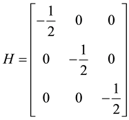
At

Hence, , and.

Therefore, is a local minimum. The value of at this point is.

For the critical points, we have

Consequently,

and

We therefore conclude that is a local maximum. The maximum value of obtained at is 0.5.

We can deduce from the result in this section and other previous works that for MA (1) process, while for MA (2) process and MA (3) process and respectively.

In what follows, we establish the bounds for, where is order of the moving average process.

Theorem 2.

Let be an MA process. Then,.

Proof

It is easily seen that for the MA process,

Partial derivatives of with respect to are as follows

Equating each of the partial derivatives to zero yields

(4.24)

From (4.24), we obtain

(4.25)

Since for an MA process, it is obvious that the equations preceding (4.24) are only satisfied if. Substituting into (4.25) leads to. The two critical points of are then and.

At, while at,. It then follows that.

Remark: For an invertible MA (3) process,. Hence, , and.

5. Conclusion

We have established necessary conditions for the parameters of an invertible MA (3) process. When the characteristic equation has three real equal roots, the conditions are, and. Also the intervals for the autocorrelation coefficients of an invertible moving average process of order three are estab-

lished. These are, and. It is also noteworthy that the

condition on for an invertible MA (3) process is generalized for of the invertible MA process. That is for the invertible MA process,. These results can now be used to compare other linear and nonlinear processes that have similar autocorrelation structures with the MA (3) process.

References

- Moses, R.L. and Liu, D. (1991) Optimal Nonnegative Definite Approximation of Estimated Moving Average Covariance Sequences. IEEE Transactions on Signal Processing, 39, 2007-2015. http://dx.doi.org/10.1109/78.134433
- Qian, G. and Zhao, X. (2007) On Time Series Model Selection Involving Many Candidate ARMA Models. Computational Statistics and Data Analysis, 51, 6180-6196. http://dx.doi.org/10.1016/j.csda.2006.12.044
- Li, Z.Y. and Li, D.G. (2008) Strong Approximation for Moving Average Processes under Dependence Assumptions. Acta Mathematica Scientia, 28, 217-224. http://dx.doi.org/10.1016/S0252-9602(08)60023-5
- Box, G.E.P., Jenkins, G.M. and Reinsel, G.C. (1994) Time Series Analysis: Forecasting and Control. 3rd Edition, Prentice-Hall, Englewood Cliffs.
- Okereke, O.E., Iwueze, I.S. and Johnson, O. (2013) Extrema of Autocorrelation Coefficients for Moving Average Processes of Order Two. Far East Journal of Theoretical Statistics, 42, 137-150.
- Al-Marshadi, A.H. (2012) Improving the Order Selection of Moving Average Time Series Model. African Journal of Mathematics and Computer Science Research, 5, 102-106.
- Adewumi, M. (2014) Solution Techniques for Cubic Expressions and Root Finding. Courseware Module, Pennsylvania State University, Pennsylvania.
- Okereke, O.E., Iwueze, I.S. and Johnson, O. (2014) Some Contributions to the Solution of Cubic Equations. British Journal of Mathematics and Computer Science, 4, 2929-2941. http://dx.doi.org/10.9734/BJMCS/2014/10934
- Wei, W.W.S. (2006) Time Series Analysis, Univariate and Multivariate Methods. 2nd Edition, Pearson Addision Wesley, New York.
- Chatfield, C. (1995) The Analysis of Time Series. 5th Edition, Chapman and Hall, London.
- Palma, W. and Zevallos, M. (2004) Analysis of the Correlation Structure of Square of Time Series. Journal of Time Series Analysis, 25, 529-550. http://dx.doi.org/10.1111/j.1467-9892.2004.01797.x
- Iwueze, I.S. and Ohakwe, J. (2011) Covariance Analysis of the Squares of the Purely Diagonal Bilinear Time Series Models. Brazilian Journal of Probability and Statistics, 25, 90-98. http://dx.doi.org/10.1214/09-BJPS111
- Iwueze, I.S. and Ohakwe, J. (2009) Penalties for Misclassification of First Order Bilinear and Linear Moving Average Time Series Processes. http://interstatjournals.net/Year/2009/articles/0906003.pdf
- Okereke, O.E. and Iwueze, I.S. (2013) Region of Comparison for Second Order Moving Average and Pure Diagonal Bilinear Processes. International Journal of Applied Mathematics and Statistical Sciences, 2, 17-26.
- Montgomery, D.C., Jennings, C.L. and Kaluchi, M. (2008) Introduction to Time Series Analysis and Forecasting. John Wiley and Sons, New Jersey.
- Sittinger, B.D. (2010) The Second Derivative Test. www.faculty.csuci.edu/brian.sittinger/2nd_Derivtest.pdf