Applied Mathematics
Vol.5 No.15(2014), Article ID:48885,26 pages
DOI:10.4236/am.2014.515227
An Asymptotic Distribution Function of the Three-Dimensional Shifted van der Corput Sequence
Jana Fialová1, Ladislav Mišk2, Oto Strauch1
1Mathematical Institute, Slovak Academy of Sciences, Bratislava, Slovakia
2Department of Mathematics, University of Ostrava, Ostrava, Czech Republic
Email: jana.fialova@mat.savba.sk, ladislav.misik@osu.cz, oto.strauch@mat.savba.sk
Copyright © 2014 by authors and Scientific Research Publishing Inc.
This work is licensed under the Creative Commons Attribution International License (CC BY).
http://creativecommons.org/licenses/by/4.0/


Received 25 May 2014; revised 1 July 2014; accepted 15 July 2014
Abstract
In this paper, we apply the Weyl's limit relation to calculate the limit

where
 is the van der Corput sequence in base
 ,
,
 is the asymptotic distribution function of
 , and
, and ,
,
 and
and , respectively.
Keywords:Sequences, Arithmetic Means, Riemann-Stieltjes Integraion

1. Introduction
In this paper we apply the Weyl’s limit relation [1] (p. 1-61)
 (1.1)
(1.1)
to the sequence , where
 is the van der Corput sequence in base
 and
and
 is the asymptotic distribution function (abbreviated a.d.f.) of
 and
and . The van der Corput sequence in base
 is defined as follows: Let
 be the
 -adic expression of a positive integer
 . Then
 (1.2)
(1.2)
It is well-known that this sequence is uniformly distributed (abbreviated u.d.), see [1] (2.11, p. 2-102), [2] (Theorem 3.5, p. 127), [3] (p. 41).
For
 a motivation for the study of the distribution function (abbreviated d.f.)
 of
of
 ,
,
 is a result of Pillichshammer and Steinerberger in [4] which states that
 (1.3)
(1.3)
while in J. Fialová and O. Strauch [5] the relation (1.3) was proved applying (1.1) as

Moreover, in the Unsolved Problems [6] (1.12),
the following problem is stated: Find the d.f.
 of the sequence
 ,
,
 , in
, in . Ch. Aistleitner and M. Hofer
[7] gave the following theoretical solution:
. Ch. Aistleitner and M. Hofer
[7] gave the following theoretical solution:
Theorem 1 Let
 denote the von Neuman-Kakutani transformation described in
Figure 1. Define the
denote the von Neuman-Kakutani transformation described in
Figure 1. Define the
 - dimensional curve
 , where
 . Then the searched
a.d.f. is
. Then the searched
a.d.f. is

where
 is the Lebesgue measure of a set
 .
.
The paper consists of the following parts: After definitions (Part 2) we derive
the a.d.f. of

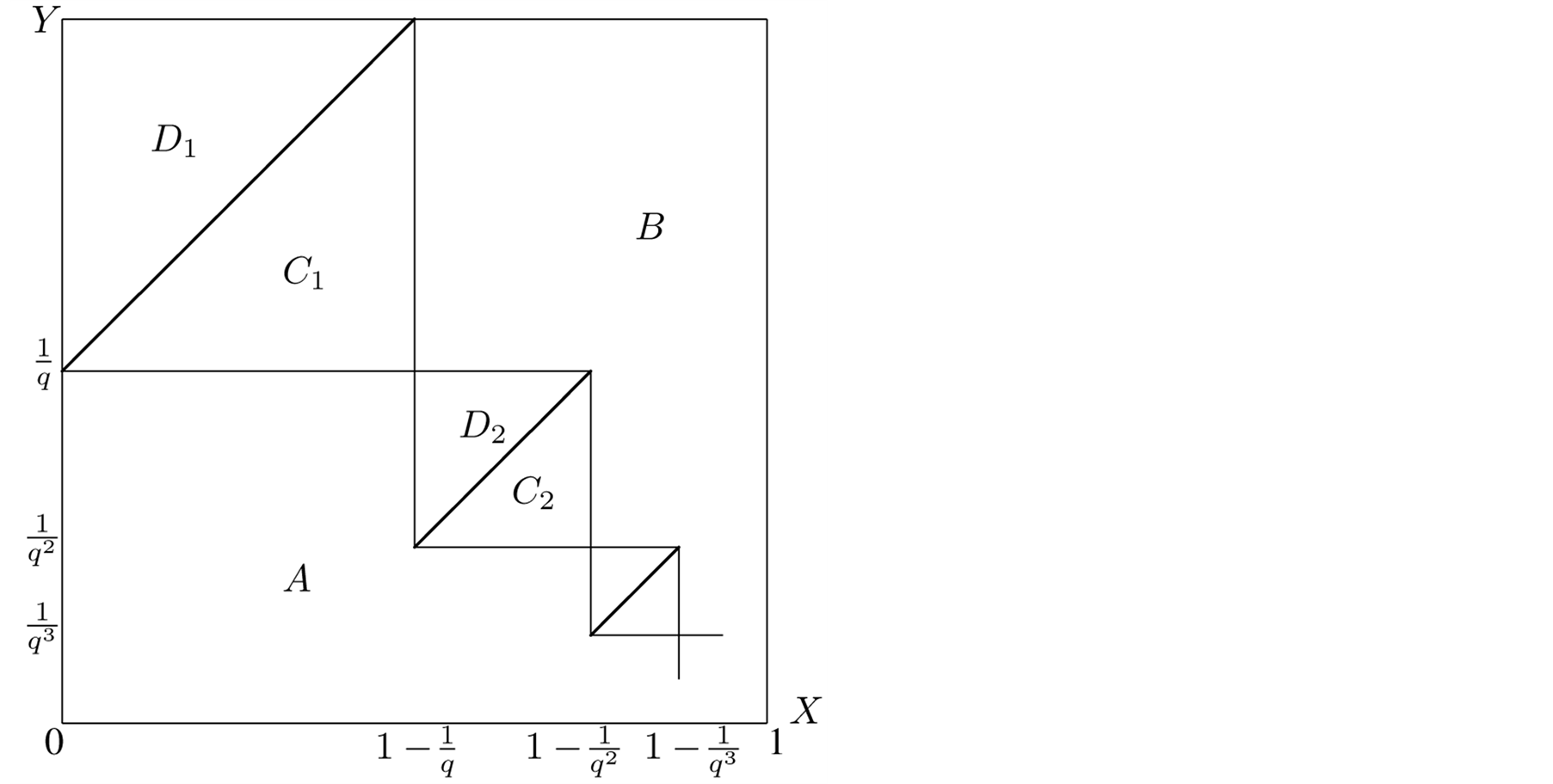
Figure 1.
Line segments containing
 The graph of the von Neumann-Kakutani transformation
 .
.
Haoshangban (Part 3), the a.d.f. of
 (Part 4), intervals containing
 in diagonals (Part 5) and an explicit form of a.d.f.
 (Part 6). As an application (Part 7) we compute
the limit
(Part 6). As an application (Part 7) we compute
the limit
 (1.4)
(1.4)
for ,
,
 and
and , respectively, see (0.39), (0.41)
and (0.46).
, respectively, see (0.39), (0.41)
and (0.46).
2. Definitions and Notations
Let ,
,
 be a sequence in the unit interval
 . Denote


the step distribution function (step d.f.) of the finite sequence
 in
in , while
 .
.
 A function
 is a distribution function (d.f.) if
(i)
 is nondecreasing;
(ii)
 and
and .
.
 A d.f.
 is a d.f. of the sequence
 ,
,
 if an increasing sequence of positive integers
 exists such that
 a.e. on
 .
.
 A d.f.
 is an asymptotic d.f. (a.d.f.) of the sequence
 ,
,
 if
if
 a.e. on
 .
.
 The sequence
 is uniformly distributed (abbreviating u.d.) if its a.d.f. is
 .
.
 Similar definitions take place for
 and
and
 -dimensional sequence
 ,
,
 , in
, in , cf.
[1] (1.11, pp. 1-60).
, cf.
[1] (1.11, pp. 1-60).
 In the sequel the
 -dimensional interval
 we denote by
 , where
 are projections on
 axes, respectively.
3. a.d.f. of
Let
 be an integer.
Lemma 1 Every point ,
,
 , lies on the diagonals of intervals
 (1.5)
(1.5)
 (1.6)
(1.6)
Proof. Express an integer
 in the base


where
 and
and . We consider the following two cases:
 ,
,
 .
.
Let
 Then
Then
 ,
,
 and by (0.2)
 . In this case

Thus such
 lies on the line-segment
 (1.7)
(1.7)
Let
 Then
Then
 and
and , where
 . Then
 . Thus
 ,
,
 , and we have
 and
and
 and
and
 . Thus such
 lies on the segment
 (1.8)
(1.8)
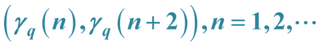
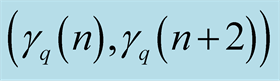
Thus, for , terms of the sequence
 lie on the diagonal of the interval
 (1.9)
(1.9)
and for , after reduction
 , terms of the sequence
 lie on the diagonals of the intervals
 (1.10)
These intervals are maximal with respect to inclusion.
Adding the maps (1.7) and (1.8) we found the so-called von Neumann-Kakutani transformation , see Figure 1.
Because
, see Figure 1.
Because
 is u.d., the sequence
 has a.d.f.
 of the form1
 (1.11)
where
 is the projection of a two dimensional set to the
 -axis.
The sum (1.11) implies
 (1.12)

From (1.12) it follows
 (1.13)
and for , the mean equality misses.
4. a.d.f. of
Let
 be an integer.
Lemma 2 All terms of the sequence ,
,
 , lie in the diagonals of the following intervals
 (1.14)
 (1.15)
 (1.16)
Proof. Express an integer
 in the base

 (1.17)
where
 and
and . We consider three following cases:
 ,
,
 ,
,
 .
.
Let
 Then
Then
 ,
,
 and
and
 . In this case
 and thus such
 lies on the line-segment
 (1.18)
Let
 . Then
 and
and , then
 . Thus
 ,
,
 , and we have
 .
.
Furthermore
 and
and
 .
.
Thus in this case
 lies on the line-segment
 (1.19)
Let .
.
Then
 and
and , then
 . Thus
 ,
,
 , and we have
 .
.
Furthermore
 and
and
 .
.
This gives
 (1.20)
Summary, if the
 satisfies
 , then
 is contained in the diagonal of
 (1.14)
for
 in the diagonal of
 (1.15)
and for
 in the diagonal of
 (1.16).
Proof. Express an integer
 in the base

 (1.17)
where
 and
and . We consider three following cases:
 ,
,
 ,
, .
.
Let
 Then
Then ,
,
 and
and . In this case
 and thus such
 lies on the linesegment
 (1.18)
Let
 . Then
 and
and , then
 . Thus
 ,
,
 , and we have
 .
.
Furthermore
 and
and .
.
Thus in this case
 lies on the line-segment
 (1.19)
Let
 . then
 and
and , then
 . Thus
 ,
,
 , and we have
 .
.
Furthermore
 and
and .
.
This gives
 (1.20)
Summary, if the
 satisfies
 , then
 is contained in the diagonal of
 (1.14) for
 in the diagonal of
 (1.15)
and for
 in the diagonal of
 (1.16).
Composition of the maps (0.18), (0.19) and (0.20) of
 forms the second iteration
 of the von Neumann-Kakutani transformation
 . The diagonals of (1.14),
(1.16) and (1.15) yield the following graph of
. The diagonals of (1.14),
(1.16) and (1.15) yield the following graph of
 in Figure 2.
Here the interval
 on
on
 -axis is decomposed in
 ,
,
 , and the interval
 is decomposed in
 ,
, . On
. On
 -axis the interval
 is decomposed in
 ,
,
 and the interval
 is decomposed in
 ,
, . Note that for
 , the interval
 has a zero length and is missing.
Exchange for a moment the axis
 by
by . Similarly as in (1.11), we have that the a.d.f.
 of the sequence
 is
is
 (1.21)
Decompose
 as the following figure shows:
Then by Figure 3 we have
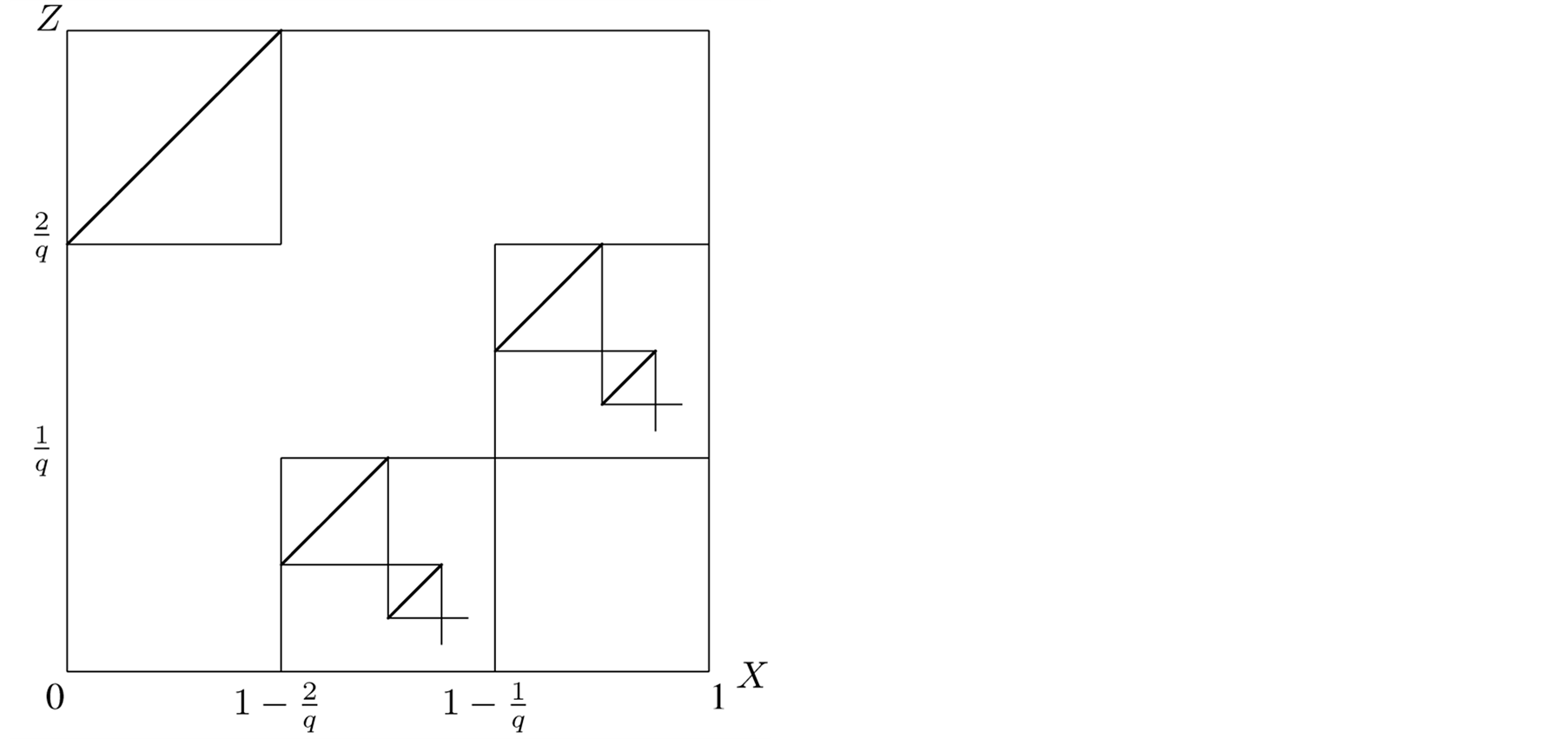
Figure 2. Straight lines
containing
 ,
, .
.
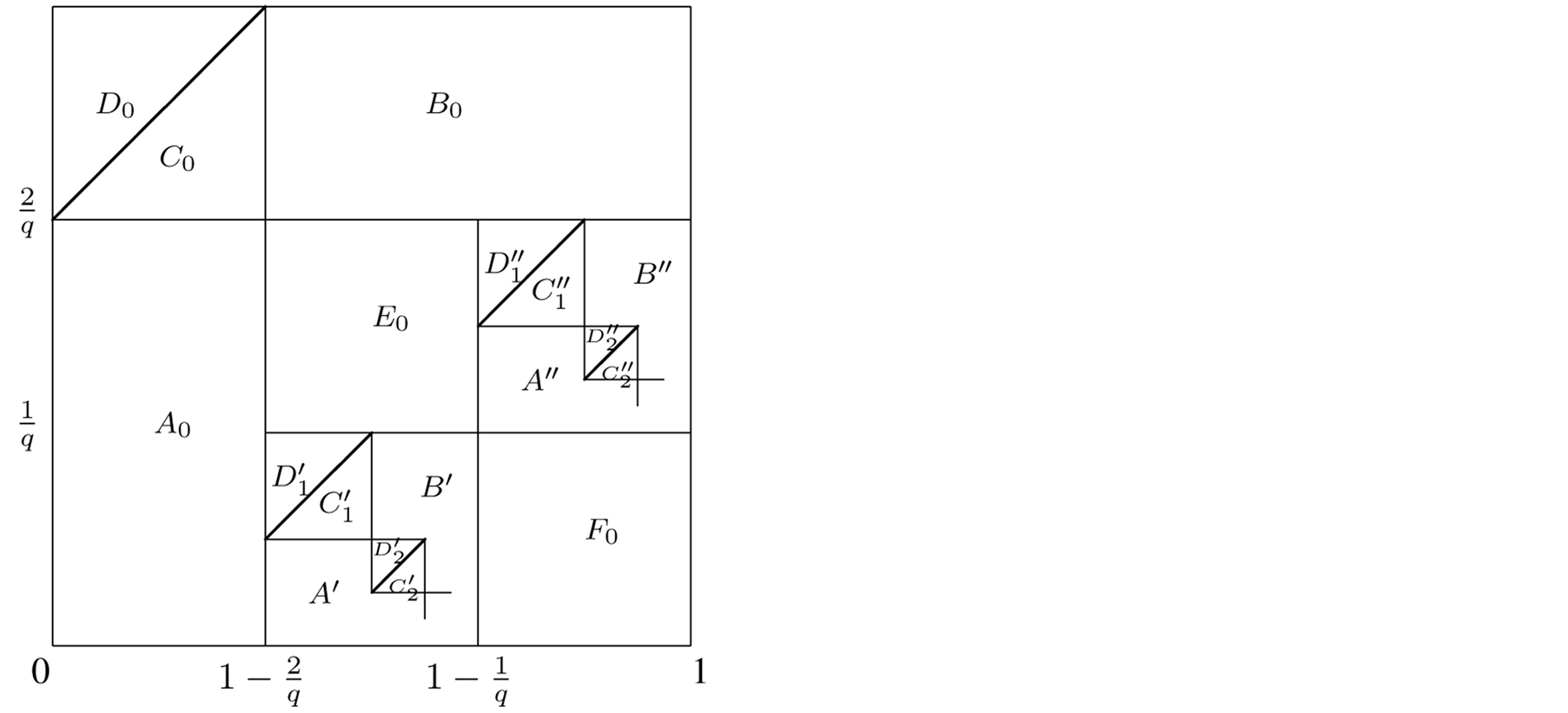
Figure 3. Decomposition of the Vunit square to parts with
fixed expression of .
.
 (1.22)
Let .
.
In this case we find a.d.f
 from (1.22) omitting

In Part 7. Applications we need to find
 from
from
 in (1.22):
For

 (1.23)
For

 (1.24)
For

 (1.25)
Note that for
 the term
 is omitted.
5. a.d.f. of
Let
 be an integer.
Lemma 3 Every point
 is contained in diagonals of the intervals
 (1.26)
 (1.27)

 (1.28)
where
 if
if . These intervals are maximal with respect to inclusion.
Proof. Every maximal
 -dimensional interval
 containing points
 will be written as
 , where
 are projections of
 to the
 , axes, respectively. Moreover if
 then
then
 and
and . From u.d. of
 follows that the lengths
 . Combining intervals (1.5),
(1.14), (1.15), (1.16), (1.6) of equal lengths by following
Figure 3.
. Combining intervals (1.5),
(1.14), (1.15), (1.16), (1.6) of equal lengths by following
Figure 3.
We find (1.26), (1.27), and (1.28).
Now, let
 be the union of diagonals of (1.27), (1.28) and (1.26). Again, as in (1.11), the
a.d.f.
be the union of diagonals of (1.27), (1.28) and (1.26). Again, as in (1.11), the
a.d.f.
 has2 the form
 (1.29)
and it can be rewritten as
 (1.30)
To calculate minimums in (1.30) we can use the following
Figure 4 (here ):
):
As an example of application of (1.30) and Figure 4,
we compute
 for
for
 without using the knowledge of
 ,3
,3
 (1.31)
Proof.
1. Let .
.
Then ,
,
 ,
,
 , consequently
 .
.
2. Let . Then
 ,
,
 ,
,
 , consequently
 .
.
3. Let . Then
 ,
,
 , consequently
 .
.
4. Let .
.
Specify ,
, . Then
 ,
,
 for
for . Thus (1.30) implies

For
 we have
 (1.32)
6. Explicit Form of
Let
 be an integer.
Motivated by the Figure 4 we decompose the unit
interval
 on
on ,
,
 and
and
 axes in the Figure 5
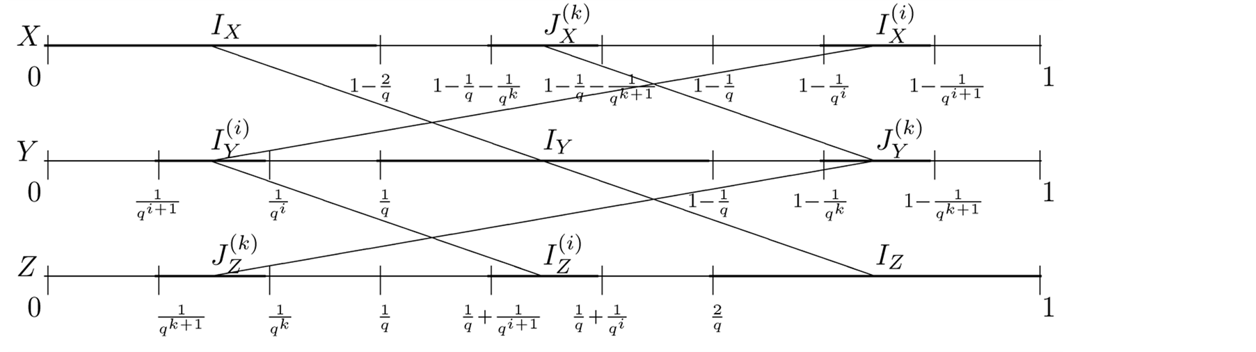
Figure 4. Projections of intervals
 on axes
 .
.
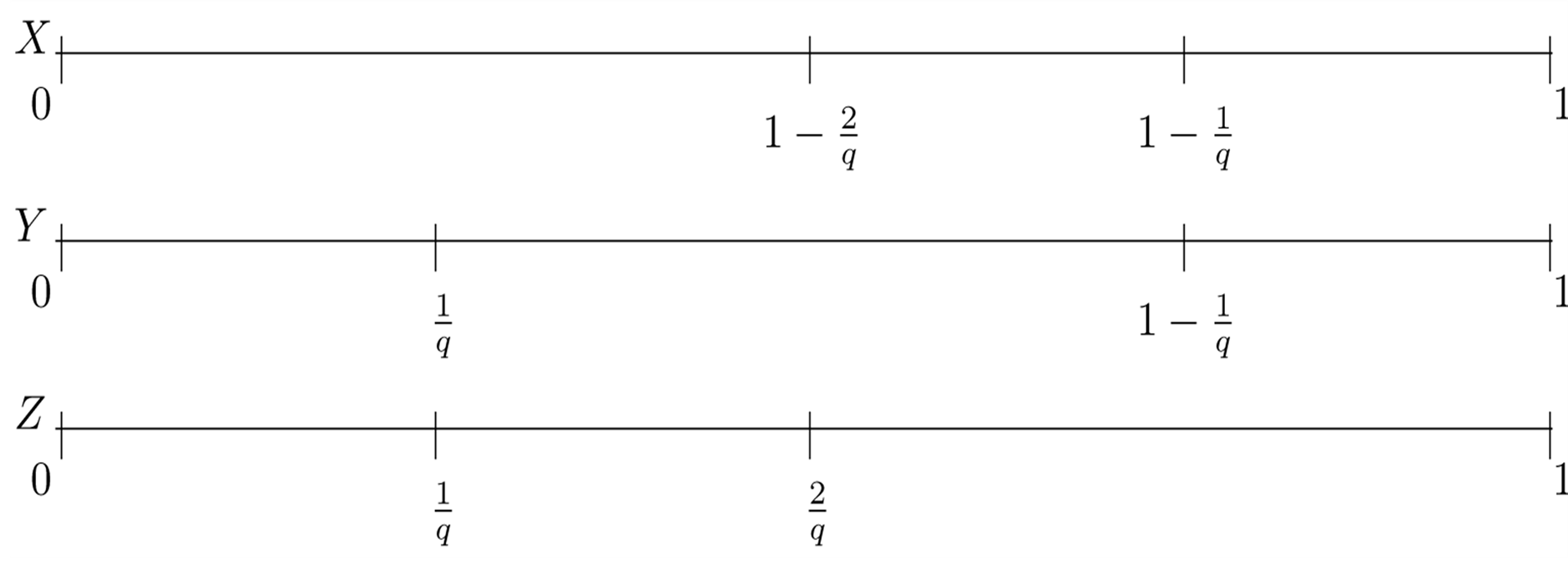
Figure 5. Divisions of the unit intervals.
intervals (here ):
):
In this decomposition, for , we have
 possibilities. We shall order choices of
 from the left to the right. Detailed proofs are included only in non-trivial cases.
1. Let
 . Then
 .
.
Proof. We have ,
,
 ,
, . Then, by (1.30),
 .
.
Similarly, in the following cases 2-9.
2. Let . Then
 .
.
3. Let . Then
 .
.
4. Let . Then
 .
.
5. Let . Then
 .
.
6. Let . Then
 .
.
7. Let . Then
 .
.
8. Let . Then
 .
.
9. Let . Then
 .
.
Proof. We use .
.
10. Let . Then
 .
.
Proof. We use ,
,
 ,
, . Similarly11. Let
 . Then
 .
.
12. Let . Then
 .
.
Proof. We use ,
,
 ,
, .
.
13. Let . Then
 .
.
14. Let . Then
 .
.
15. Let . Then
 .
.
16. Let .
.
Specify ,
,
 ,
, . Then

Proof. First observe that , and
, and . Thus
 and
and

Further, for , we have


Thus, using (1.30), we find
 .
.
17. Let .
.
Specify ,
, . Then

Proof. We have ,
,
 ,
,
 , then

18. Let .
.
Specify ,
, . Then

Proof. We have

19. Let . Then
 .
.
20. Let .
.
Specify ,
,
 ,
, . Then we have

Proof. We have ,
,
 and
and

21. Let .
.
Specify ,
, . Then

Proof. ,
,
 ,
,
 ,
,

22. Let . Then
 .
.
23. Let .
.
Specify ,
, . Then

Proof. ,
,
 ,
,
 ,
,

24. Let . Then
 .
.
Proof. We have . Specify
 . Then

The first term is
 and the second is
 .
.
25. Let .
.
Specify ,
, . Then

Proof.

26. Let .
.
Specify ,
,
 and
and . Then

Proof. We have ,
,
 ,
,
 ,
, . Moreover


which gives
 .
.
The final equation holds if
 and
and . It can be seen that it holds also for
 and
and . For
. For
 and
and
 we need to compute this sum separately.
27. Let . Then
 .
.
Proof. First observe
 ,
,
 ,
, . Thus
 .
.
New specify
 and
and . Then we have


and ,
,
 ,
, . Then for the sums in (1.30)
we have
. Then for the sums in (1.30)
we have

which gives .
.
The above computation of
 holds for
 .
.
Let .
.
We have
 and
and
 (1.33)
Thus
 for
for
 directly follows from
 for
for
 if we use only such items in
 for which
 ,
,
 ,
, . These are
 , i.e.,
 .
.
The non-zero values of
 can also be seen in the following table.
In all other cases .
.
7. Applications
The knowledge of the a.d.f.
 of the sequence

 allows us to compute the following limit by the Weyl limit relation (1.1) in dimension
 .
.
 (1.34)
where
 is an arbitrary continuous function defined in
 . For computing (1.34)
we use the following two methods.
. For computing (1.34)
we use the following two methods.
7.1. Method I
In the first method in the Riemann-Stieltjes integral (1.34) we apply integration by parts.
Lemma 4 Assume that
 is a continuous in
 and
and
 is a.d.f. Then
 (1.35)
Here
 (1.36)
Note that


if the partial derivatives exist.
Exercise 1 Put . We have
 ,
,
 The differential
 is non-zero if and only if
 and in this case
 .
.
Proof: For every interval
 and every continuous
 the differential
 is defined as
 (1.37)
Putting ,
,
 ,
,
 we have

Then by (1.35)
 (1.38)
For
 and by (1.31) we have

For
 and by (1.32) we have

Therefore for , by (1.34) and by (1.38) we
have
, by (1.34) and by (1.38) we
have
 (1.39)
Note that the same result follows from (1.44).
Exercise 2 Put . Since
 ,
,
 if
if ,
,
 if
if ,
,
 if
if , and
, and
 if
if
 and
and
 otherwiseapplying (1.34) and (1.35) we have
 (1.40)
Here we have
 in (1.13) for
 . For
. For
 we use
 in (1.23) if
 , (1.24) if
 and (1.25) if
 and for
 we use (1.31) if
 and (1.32) if
 . Thus we have:
a)
 for
for ;
;
b)
 for
for ;
;
c)
 for
for ;
;
d)
 for
for .
.
e)
 for
for ;
;
f)
 for
for .
.
Putting a)-f) into (1.40) yields
 (1.41)
7.2. Method II
In the second method we compute the differential
 directly. It is nonzero only for
 . For such
 the a.d.f.
 has the form
 (1.42)
Thus
 and moreover
 only on the following straight lines


Considering three possible cases, calculate
 (1.43)
Summary
 (1.44)
Exercise 3 Put . By Method I, we
have
. By Method I, we
have , similarly
 , etc., and by
(1.35) we have
, etc., and by
(1.35) we have
 (1.45)
Since a computation of (1.45) is complicated we use Method II, by (1.44) we have

Inserting these formulas into (1.44) we have
 (1.46)
for .
.
8. Conclusion
The problems solved in this paper is significantly more complicated in higher dimensions . For example, in dimension
 , to compute the d.f.
 of the sequence
 , it is necessary to
investigate
, it is necessary to
investigate
 cases analogous to
 cases for the explicit form
 in the part 0.6. Also Figure 3 would have to be
converted to the dimension
in the part 0.6. Also Figure 3 would have to be
converted to the dimension . Finally, we would need
the third iteration of von Neumann-Kakutani transformation.
. Finally, we would need
the third iteration of von Neumann-Kakutani transformation.
Acknowledgements
The paper is sponsored by the project P201/12/2351 of GA Czech Republic.
References
- Strauch, O. and Porubsky, S. (2005) Distribution of Sequences: A Sampler. Peter Lang, Frankfurt am Main. (Electronic Revised Version December 11, 2013) https://math.boku.ac.at/udt/books/MYBASISNew.pdf
- Kuipers, L. and Niederreiter, H. (1974) Uniform Distribution of Sequences. John Wiley (reprint edition published by Dover Publications, Inc., Mineola, New York in 2006). https://math.boku.ac.at/udt/books/KuipersNiederreiter
- Drmota, M. and Tichy, R.F. (1997) Sequences, Discrepancies and Applications. Springer Verlag, Berlin.
- Pillichshammer, F. and Steinerberger, S. (2009) Average Distance between Consecutive Points of Uniformly Distributed Sequences. Uniform Distribution Theory, 4, 51-67. https://math.boku.ac.at/udt/vol04/no1/Pilli-Stein09-1.pdf
- Fialová, J. and Strauch, O. (2011) On Two-Dimensional Sequences Composed of One-Dimensional Uniformly Distributed Sequences. Uniform Distribution Theory, 6, 101-125. https://math.boku.ac.at/udt/vol06/no1/8FiSt11-1.pdf
- Strauch, O. (2013) Unsolved Problems. Tatra Mountains Mathematical Publications, 56, 109-229.http://www.boku.ac.at/MATH/udt/unsolvedproblems.pdf
- Aisleitner, Ch. and Hofer, M. (2013) On the Limit Distribution of Consecutive Elements of the van der Corput Sequence. Uniform Distribution Theory, 8, 89-96. https://math.boku.ac.at/udt/vol08/no1/08AistHofer37-11.pdf
NOTES

1 is a copula.