Applied Mathematics
Vol.4 No.3(2013), Article ID:29085,10 pages DOI:10.4236/am.2013.43079
Optimal Production Control of Hybrid Manufacturing/Remanufacturing Failure-Prone Systems under Diffusion-Type Demand
Mechanical Engineering Department, École de Technologie Supérieure, Montreal, Canada
Email: samir.ouaret.1@ens.etsmtl.ca, vladimir.polotski@etsmtl.ca, jean-pierre.kenne@etsmtl.ca, ali.gharbi@etsmtl.ca
Received October 14, 2012; revised January 31, 2013; accepted February 7, 2013
Keywords: Stochastic Control; Manufacturing Systems; Optimization; Failure; Random Process
ABSTRACT
The problem of production control for a hybrid manufacturing/remanufacturing system under uncertainty is analyzed. Two sources of uncertainty are considered: machines are subject to random breakdowns and repairs, and demand level is modeled as a diffusion type stochastic process. Contrary to most of studies where the demand level is considered constant and fewer results where the demand is modeled as a Poisson process with few discrete levels and exponentially distributed switching time, the demand is modeled here as a diffusion type process. In particular Wiener and OrnsteinUhlenbeck processes for cumulative demands are analyzed. We formulate the stochastic control problem and develop optimality conditions for it in the form of Hamilton-Jacobi-Bellman (HJB) partial differential equations (PDEs). We demonstrate that HJB equations are of the second order contrary to the case of constant demand rate (corresponding to the average demand in our case), where HJB equations are linear PDEs. We apply the Kushner-type finite difference scheme and the policy improvement procedure to solve HJB equations numerically and show that the optimal production policy is of hedging-point type for both demand models we have introduced, similarly to the known case of a constant demand. Obtained results allow to compute numerically the optimal production policy in hybrid manufacturing/ remanufacturing systems taking into account the demand variability, and also show that Kushner-type discrete scheme can be successfully applied for solving underlying second order HJB equations.
1. Introduction
In recent years, the reverse logistics framework allowing the unified analysis of manufacturing planning and the inventory management has gained a substantial interest among the researchers working in the field. In a book [1] author described the quantitative models to represent the activities of remanufacturing and recycling in the context of reverse logistics emphasizing three issues: namely: distribution planning, inventory management and production planning. In the survey [2] authors analyzed more than sixty case studies in reverse logistics published between 1984 and 2002 and discussed network structures and activities related to the recovery of products up to the end of life. Various optimization models for supply chains with a recovery of returned products have been proposed with special attention to the production control and inventory management using both, deterministic and stochastic approaches. In the majority of previous studies discrete time (as opposed to continuous time) settings is used. In [3] authors present an effective approach to determine the discrete policy of the optimal control for a system with product recovery, taking into account the uncertainty in the demand of new and returned products. They model the demand and the return as discrete independent random variables. In [4] a new discrete stochastic inventory model for a hybrid system is proposed: new and returned products are manufactured separately, the demands are independent but production policies are synchronized. Authors of [5] develop a periodic inventory model of on a finite planning horizon with consideration of production remanufacturing and disposal activities. In [6] authors propose a model of discrete time stochastic optimization for a hybrid system taking into account, the production, subcontracting, remanufacturing of returned products, return market of poor quality products the production line and disposal activities. The demand is a random variable normally distributed and the return of products depends on the demand. A continuous time optimization model is considered in [7] for the production, remanufacturing and disposal in a dynamic deterministic settings.
Manufacturing systems subject to random breakdowns and repairs were systematically analyzed in [8-10] in continuous time using stochastic optimization technique. Recently in [11] this methodology has been extended to address the global performances of the manufacturing system with the supply chain in closed loop. A stochastic dynamic system consisted of two machines dedicated respectively to manufacturing and remanufacturing; the random phenomena are breakdowns and repairs of the machines, the demand of new products was considered deterministic and known, the returned product was a portion of this demand.
The constant demand is a prevailing assumption in the large body of the research devoted to stochastic continuous time optimization of production management in failure-prone systems. Some papers develop optimality conditions and use them for searching numerical solutions [12]; others present analytical solutions as the recent article [13]. In much fewer studies where the random demand is analyzed—it is most often modeled as a Poisson process. This approach allows to keep the usual framework of random discrete events changing the state of the system for both machine breakdowns and demand jumps [14]. Poisson-type demand is used more systematically in inventory optimization problems [15]. A combined model: Poisson process coupled with the diffusion process has been recently proposed in [16] for modeling the demand in inventory problem. In fact diffusion-type processes were used for modeling the demand in the classical paper [8] were optimality conditions have been obtained, however it was the only source of random behavior since the machine breakdowns were not considered.
The system considered in this paper contains reverse logistics loop with manufacturing and remanufacturing branches revisiting the model proposed in [14]. We use continuous time stochastic control approach and adopt the diffusion-type component into the demand model merging this source of random behavior with random machine breakdowns described by Poisson process as in [9,10]. As a direct consequence of an adopted demand model the optimality conditions lead to the HamiltonJacobi-Bellman (HJB) equation of the second order. Second order HJB is often met in option price modeling, but for stochastic control in manufacturing systems the HJB is usually of the first order [9,10,14]. Analyzing the second order HJB we use the Kushner finite difference approximations and the policy improvement algorithm [17].
The paper is structured as follows. In Section 2 we describe the model of the hybrid system consisting of 2 machines. The first machine uses primary product, and the second—returned product; both are subject to breakdowns and repairs constituting the first source of uncertainty. We describe in details our demand model using diffusion type random processes constructed as an output of shaping filter excited by the white noise. We study 2 versions of such model simple Brownian motion and first order Markovian process. Latter version seems more realistically fit the real world situations. In Section 3 we derive optimality conditions in the form of Hamilton-Jacobi-Bellman (HJB) equations which are second order partial differential equations (PDEs) for the chosen demand model. In Section 4 we describe the numerical method based on finite difference approximations and policy improvement approach following the methodology proposed in [17] and also in [12]. In Section 5 we apply the developed methodology to the manufacturing system described in Section 2, compute the optimal production policy and show that it is of classical hedging point type. In conclusion we discuss the proposed methodology and obtained results, and outline the possible directions for future works.
2. Model of a Hybrid Manufacturing System Suitable for Stochastic Control
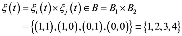
We consider a hybrid manufacturing/remanufacturing system consisting of two parallel machines denoted M1 and M2 respectively, producing the same type of product. Stochastic phenomena are demand level and machine breakdowns/repairs. We take into account the activity of production in forward direction and the activity of reutilization of returned products in reverse logistics. The demand must be satisfied by inventory for serviceable items. This inventory will be built by the products manufactured or reused. The returned products will be in the second inventory namely recovery, they can be remanufactured, or be hold on stock for future remanufacturing. In our problem, we assume that the maximal production rates for each machine are known and the machine M2 is producing at average supply for return rate, which is also its maximal rate. This situation is illustrated in Figure 1. State of the machine  with
with  is modeled as a Markov process in continuous time with discrete state
  (
( —machine is operational,
 —machine is out of order). We may the define
State transition diagram is shown in Figure 2.
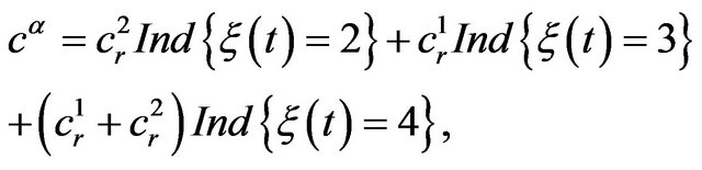
Hybrid system is in production while in modes 1, 2 and 3. Transition probabilities from state  to state
  for machine
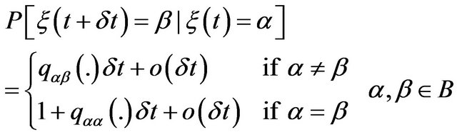 (1)
(1)
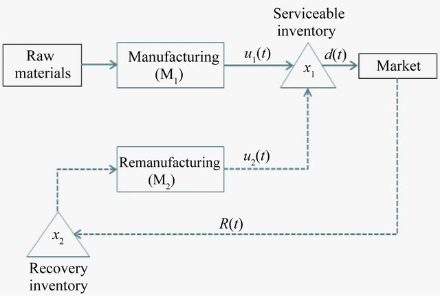
Figure 1. System structure.
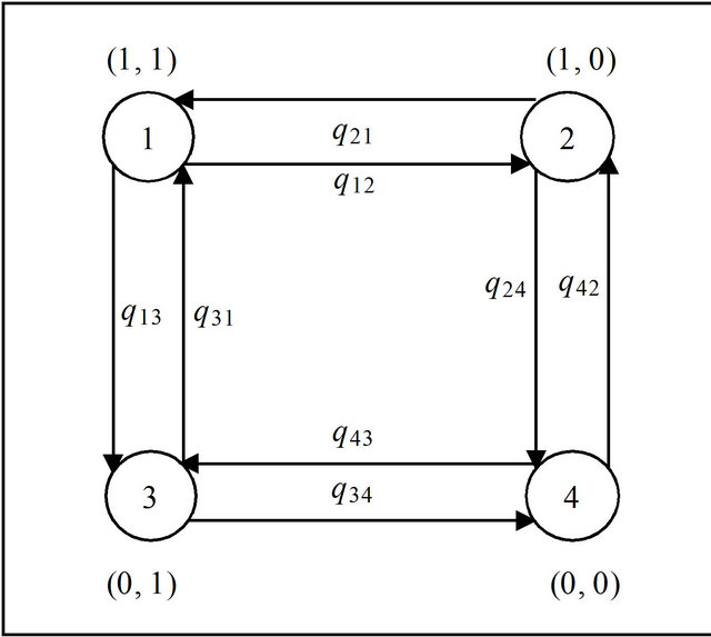
Figure 2. State transition diagram.
With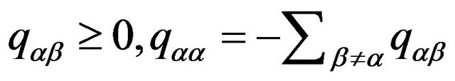 ,
, 
State transition (4 × 4) matrix  is therefore given by
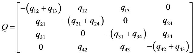
(2)
State equations can be written in the simplified form
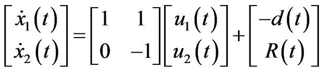 (3)
(3)
Since the demand  and return
  rates are considered as stochastic processes the more rigorous Ito form of Equations (3) will be used later. Namely let d(t) be a stationary Gaussian process with the constant mean and variance
 , where
 . Below we further specify
  in one of two ways: either an increment of a standard Brownian motion, or an increment of the first order Markov process defined later using the shaping filter.
For the return (remanufacturing) rate, an assumption is made that it is proportional to the customer demand rate 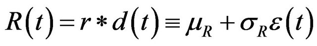 with r is a percentage of return.
Stochastic state differential Equations (3) can be rewritten in Ito form using notation 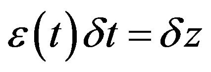
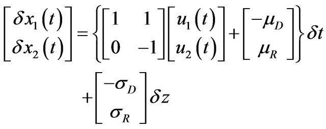 (4)
(4)
Equations (4) will be also used in the following generic form:
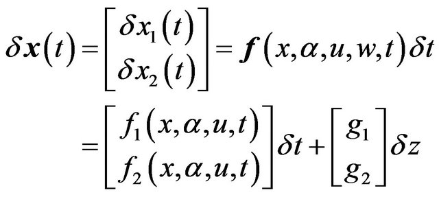 (5)
(5)
For the Case A the input  to Equations (4) is specified as a standard Brownian motion increment
  .
.
For the Case B the input  to (4) is specified as an increment of the shaping filter output (Ornstein-Uhlenbeck process)
 where
where  (6)
(6)
Process  is a first order Markovian, its correlation function is
 .
.
Additional insight to the proposed demand model can be given by considering the cumulative demand:  where
where  is a constant demand ramp,
  is a randomly varying portion of the demand. For the case A.
  (Wiener process), for the case B.
  (Ornstein-Uhlenbeck process). Also case A can be obtained from B setting
 .
.
Following constraints have to be added to (5)-(6)
 (7)
(7)
Let the cost rate function to be defined as follows:
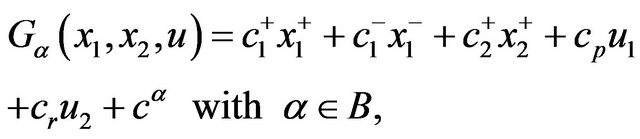 (8)
(8)
Here ,
, 
 : inventory holding and backlog costs for manufactured product (per time unit);
 : inventory holding cost for remanufactured product (per time unit);
 : production costs for manufacturing and remanufacturing processes (per unit);
 : maintenance cost for nonoperational state of the machines:
where
The objective is to determine the production rates  and
and  in order to minimize the expected discounted cost (
 is the discount rate):
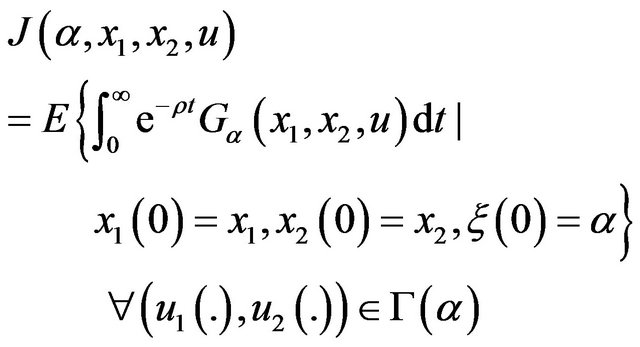 (9)
(9)
The domain  of admissible controls is defined as
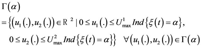 (10)
(10)
Defined hybrid system is said to be meeting feasibility condition if
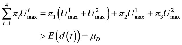 (11)
(11)
where  et
et  are limiting probabilities and maximal productions rates. We recall that the vector of limiting probabilities is defined as an eigenvector of the transition matrix Q(.)
 et
et  (12)
(12)
3. Optimality Conditions for Stochastic Control Problem
Let us define the value function is defined as a minimum (infimum) of expression (9) over all possible control inputs:
 (13)
(13)
Let us briefly recall the guidelines for obtaining optimality conditions. Introducing time-dependant α-dependant cost function and value function we have:
 (14)
(14)
According to Bellman optimality principle for cost function at  we can write
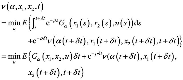
(15)
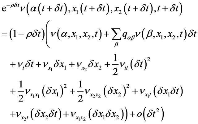
Using Taylor expansion for the term  and the value function
  over last 3 arguments, and keeping linear terms over
  and up to second order terms over
  we get:
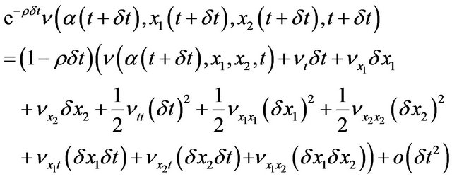
(16)
Second order terms over  are kept for further analysis because of diffusion-type processes affecting system dynamics. One more technical step consists of computing the value function
  using Markov chain-type machine dynamics (2) defined through transition probabilities
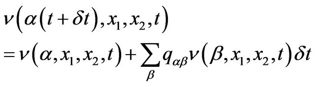 (17)
(17)
Merging Equations (16) and (17) we get
 (18)
(18)
Averaging over random realizations of the demand driven by the Brownian input  using Equations (5) and applying Ito’s lemma we get:
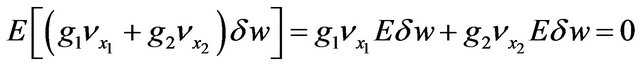
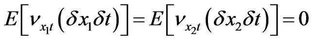
Now neglecting all terms of order higher than 1 over
 taking
 , and considering the stationary regime
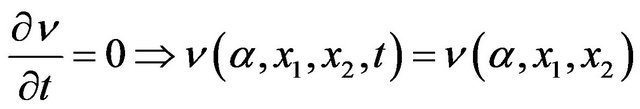 , we finally get HJB equations in the following form:
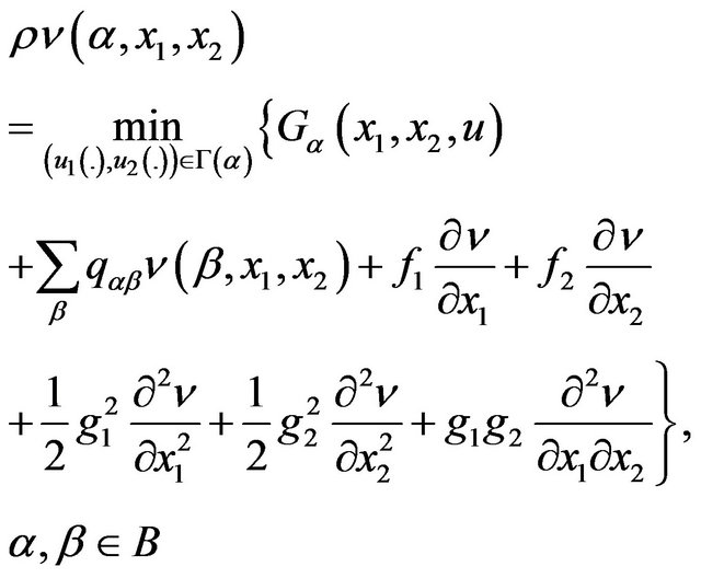 (19)
(19)
4. Numerical Method—Policy Improvement
A numerical approach proposed by Kushner in [17] and successfully used in the series of works [9,12] consists of introducing the grid in the state space  for approximating the value function
  approximating the first derivatives by “up wind” finite differences, then use policy improvement—discrete analog of a gradient descent in policy (control) space. Use of “up-wind” derivatives results in conditional computations but greatly improve convergence of the numerical.
4.1. Computations of First Derivative
To describe conditional computations of the derivatives let us introduce the following notation:
with 
The first derivatives of the value function with respect to  and
and  are:
are:
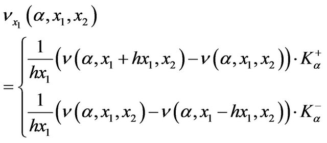 (20)
(20)
 (21)
(21)
It worth emphasizing that there is no conditional computation for  since
since  all the time due to assumption described in Section 2.
4.2. Computations of Second Derivatives
For  and for
  we have
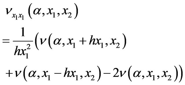 (22)
(22)
 (23)
(23)
Both expressions above do not need conditional computations, contrary to the cross derivative  which might need up to four different schemes. Since the return inventory is always positive we will use just two schemes (main inventory can be positive or negative).
If  and
and  we have
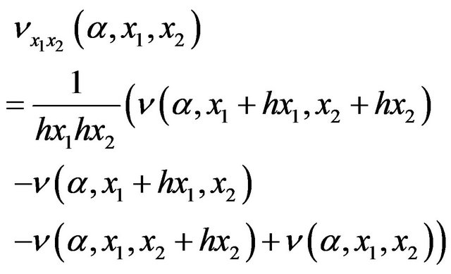 (24)
(24)
If  and
and  we have
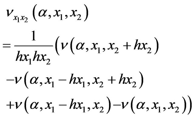 (25)
(25)
As a result we obtain for the case of Brownian motion the following discrete HJB equations:
In mode 1: ; we obtain:
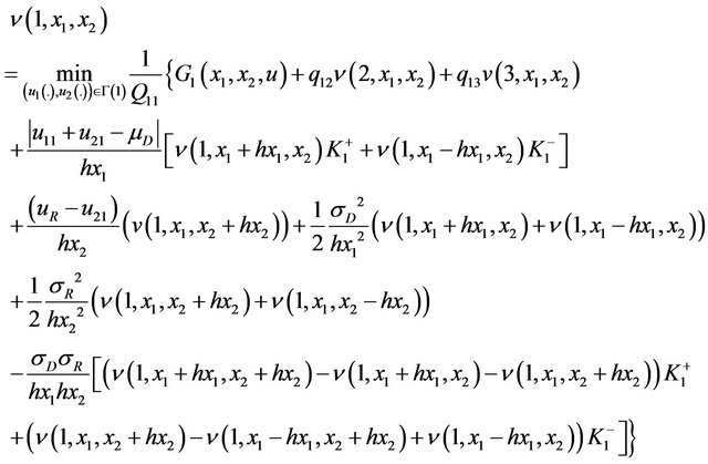 (26)
(26)
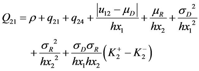
Mode 2: ;
;  and
and
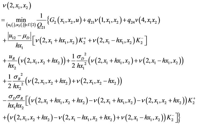 (27)
(27)
Mode 3: ;
;  and
and
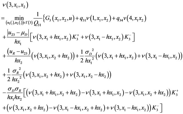 (28)
(28)
Mode 4: ;
;  and
and ,
,  and the value function
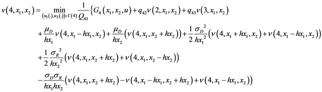 (29)
(29)
where:
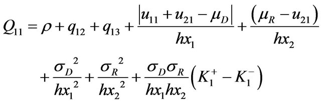 (30)
(30)
 (31)
(31)
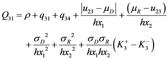 (32)
(32)
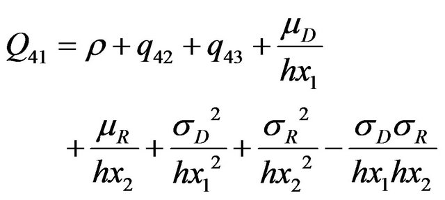 (33)
(33)
In the second case (filter demand) we have similar HJB equations in four modes, but with slightly different parameters in the first derivative of the value function namely: 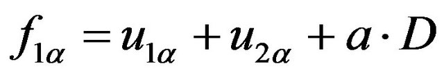 and
and 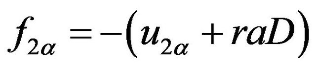 .
.
5. Optimal Production Policy for Hybrid System-Simulation Results
The first case we have analyzed corresponds to the hybrid system with manufacturing costs set relatively high in order to enforce production in remanufacturing loop. The (cumulative) demand is modeled as a Brownian process. The results are shown in Figures 3-6. Figure 3 illustrates the shape of the value function 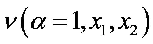 depending on the stock levels of manufactured
  and remanufactured
  products in mode 1. Value functions in other modes have similar shapes and are not shown. Figures 4 and 5 illustrate the optimal policy for the machine 1 (manufacturing) in mode 1 (both machines in operation) and mode 2 (remanufacturing machine 2 in failure) respectively. The optimal policies for the machine 1 are of hedging-point type, namely: maximal production if the stock level
  is below the threshold, zero production above the threshold and production “on demand” at the threshold-level. Comparing Figures 3 and 4 one can observe that the threshold level in mode 2 when machine 2 is in failure is higher than in mode 1.
Figure 6 illustrates the optimal policy for the machine
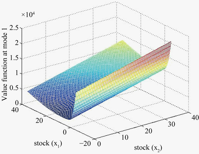
Figure 3. Value function in mode 1.
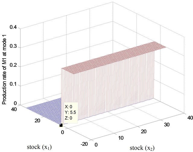
Figure 4. Production policy: Machine 1, mode 1.
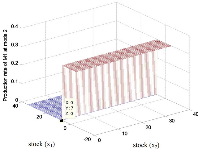
Figure 5. Production policy: Machine 1, mode 2.
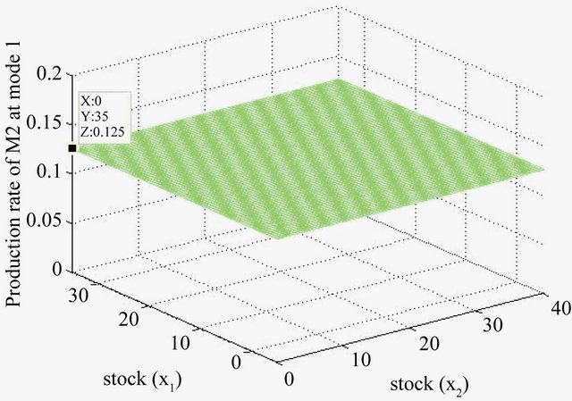
Figure 6. Production policy: Machine 2, mode 1.
2 (remanufacturing) in modes 1 when both machines are in operation (optimal policy of the machine 2 in mode 3 is identical). Machine 2 is must produce at average supply (proportional to demand) rate—which is also its maximal rate as explained in the section 2.
Figures 7 and 8 show the realizations of Brownian and Markov-type (filtered) demand rates respectively (the variance  is set to the same value). Comparing two graphs one can see that in Brownian case (Figure 7) the variation rate is much faster than in Markov case (Figure 8).
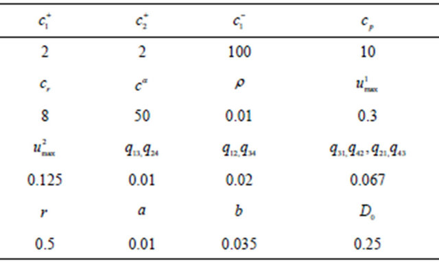
Figures 9 and 10 illustrate the optimal policy for the machine 1 (manufacturing) in mode 1 (both machines in operation) and mode 2 (remanufacturing machine 2 in failure) respectively. The results are to be compared with those shown in Figures 4 and 5. One can observe that the threshold values for the case of slower varying Markov demand are lower as compared to the case of Brownian demand. Parameters used for simulations are summarized in Table 1.
In the second case of Markov-type (filtered) demand the parameters of the filter may be used to fit the model
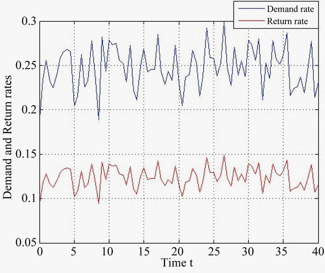
Figure 7. Brownian demand and return rates.
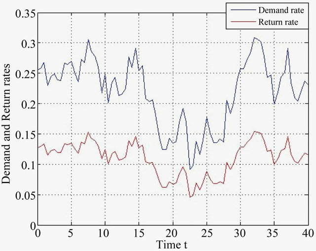
Figure 8. Filtered demand and return rates.
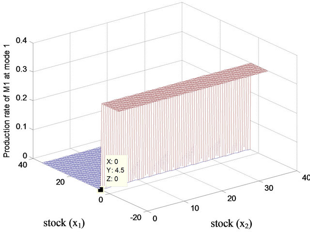
Figure 9. Production policy: Machine 1, mode 1.
to the characteristics observed in the real life applications. A classical assumption of the constant demand in this context means that the variability of the demand is ignored and only its average rate is taken into account. A

Figure 10. Production policy: Machine 1, mode 2.
Table 1. Parameters of the numerical example.
second order terms in HJB equations reflecting demand variability are in that case neglected and the optimal policy is found using the first order approximation of HJB equation. Optimal policy for the main (manufacturing) machine is of hedging point in both studied (Brownian and Markov) cases—as it is for the constant demand. According to Figures 4, 5, 9 and 10 one can see that more the demand varies rapidly in time, more the hedging stock level increases in order to respond to the demand variability. In addition, the average total cost also increases from 1939 (Markov) to 2236.5 (Brownian) as the demand variability increases.
6. Conclusion and Future Work
We have shown that the problem of stochastic control corresponding to optimization of production planning in failure prone hybrid manufacturing/remanufacturing systems with random demand can be successfully analyzed for diffusion-type demands. We investigate this problem in continuous time which seems to be the most natural setting. We develop optimality conditions in the form of HJB equations and show that due to the Brownian component in the demand the HJB equations are the second order PDEs, contrary to the case of a constant demand where they are of the first order. We use finite difference approximations for HJB equations reducing a continuous time optimization problem to the discrete time, discrete state, infinite horizon dynamic programming problem, and use policy improvement technique [17] for solving it. Value functions of the stochastic optimization problems are usually non-smooth and corresponding HJB equations have to be addressed using generalized approaches such as viscosity solutions [18]. Theoretical studies of the convergence of discrete approximations to an exact (viscosity-type) solution of HJB equations when the size of the grid tends to zero is addressed in [19,20]. Such theoretical analysis is out of the scope of this paper where we propose a numerical approach targeting the new model for the uncertain demand that allows addressing more naturally the growing number of industrial applications. Considering possible extensions of the study presented in this paper we count to explore a compound demand model of Poisson and diffusion-type process thus allowing both the jumps and continuous random variation of the demand.
REFERENCES
- M. Fleischmann, “Quantitative Models for Reverse Logistics,” Springer Verlag, New York, 2001. doi:10.1007/978-3-642-56691-2
- M. P. De Brito, R. Dekker and S. D. P. Flapper, “Reverse Logistics: A Review of Case Studies,” ERIM Report Series Reference No. ERS-2003-012-LIS, 2003.
- G. P. Kiesmüller and C. W. Scherer, “Computational Issues in a Stochastic Finite Horizon One Product Recovery Inventory Model,” European Journal of Operational Research, Vol. 146, No. 3, 2003, pp. 553-579. doi:10.1016/S0377-2217(02)00249-7
- K. Inderfurth, “Optimal Policies in Hybrid Manufacturing/Remanufacturing System with Product Substitution,” International Journal of Production Economics, Vol. 90, No. 3, 2004, pp. 325-343. doi:10.1016/S0925-5273(02)00470-X
- M. E. Nikoofal and S. M. M. Husseini, “An Inventory Model with Dependent Returns and Disposal Cost,” International Journal of Industrial Engineering Computations, Vol. 1, No. 1, 2010, pp. 45-54.
- S. Oscar and F. Silva, “Suboptimal Production Planning Policies for Closed-Loop System with Uncertain Levels of Demand and Return,” The 18th IFAC World Congress, Milano, 28 August-2 September 2011.
- I. Dobos, “Optimal Production-Inventory Strategies for HMMS-Type Reverse Logistics System,” International Journal of Production Economics, Vol. 81-82, 2003, pp. 351-360. doi:10.1016/S0925-5273(02)00277-3
- W. H. Fleming, H. M. Soner and S. P. Sethi, “A Stochastic Production Planning Problem with Random Demand,” SIAM Journal on Control and Optimization, Vol. 25, No. 6, 1987, pp.1494-1502. doi:10.1137/0325082
- E. K. Boukas and A. Haurie, “Manufacturing Flow Control and Preventive Maintenance: A Stochastic Approach,” IEEE Transactions on Automatic Control, Vol. 33, No. 9, 1990, pp. 1024-1031. doi:10.1109/9.58530
- J. P. Kenné and E. K. Boukas, “Hierarchical Control of Production and Maintenance Rates in Manufacturing Systems,” Journal of Quality in Maintenance Engineering, Vol. 9, No. 1, 2003, pp. 66-82. doi:10.1108/13552510310466927
- J. P. Kenné, P. Dejax and A. Gharbi, “Production Planning of a Hybrid Manufacturing-Remanufacturing System under Uncertainty within a Closed-Loop Supply Chain,” International Journal of Production Economics, Vol. 135, No. 1, 2012, pp. 81-93. doi:10.1016/j.ijpe.2010.10.026
- H. Yan and Q. Zhang, “A Numerical Method in Optimal Production and Setup Scheduling of Stochastic Manufacturing Systems,” IEEE Transaction on Automatic Control, Vol. 42, No. 10, 1997, pp. 441-449. doi:10.1109/9.633837
- E. Khemlnitsky, E. Presman and S. P. Sethi, “Optimal Production Control of a Failure-Prone Machine,” Annals of Operations Research, Vol. 182, 2011, pp. 67-86. doi:10.1007/s10479-009-0668-3
- J. R. Perkins and R. Srikant, “Failure-Prone Production Systems with Uncertain Demand,” IEEE Transaction on Automatic Control, Vol. 46, No. 3, 2001, pp. 441-449. doi:10.1109/9.911420
- E. Presman and S. P. Sethi, “Inventory Models with Continuous and Poisson Demands and Discounted and Average Costs,” Production and Operations Management, Vol. 15, No. 2, 2006, pp. 279-293. doi:10.1111/j.1937-5956.2006.tb00245.x
- A. Bensoussan, R. Liu and S. P. Sethi, “Optimality of an (s, S) Policy with Compound Poisson and Diffusion Demands: A Q.V.I. Approach,” SIAM Journal of Control and Optimization, Vol. 44, No. 5, 2005, pp. 1650-1676. doi:10.1137/S0363012904443737
- H. J. Kushner and P. Dupuis, “Numerical Methods for Stochastic Control Problems in Continuous Time,” Springer Verlag, New York, 1992. doi:10.1007/978-1-4684-0441-8
- W. H. Fleming and H. M. Soner, “Controlled Markov Processes and Viscosity Soutions,” Springer Verlag, New York, 2005.
- G. Barles and E. R. Jakobsen, “On the Convergence Rate of Approximation Schemes for HJB Equations,” Mathematical Modeling and Numerical Analysis, Vol. 36, No. 1, 2002, pp. 33-54. doi:10.1051/m2an:2002002
- N. V. Krylov, “On the Rate of Convergence of Finite-Difference Approximations for Bellman’s Equations with Variable Coeffcients,” Probability Theory and Related Fields, Vol. 117, No. 1, 2000, pp. 1-16. doi:10.1007/s004400050264