Applied Mathematics
Vol. 3 No. 11 (2012) , Article ID: 24519 , 8 pages DOI:10.4236/am.2012.311234
Exact Distributions of Waiting Time Problems of Mixed Frequencies and Runs in Markov Dependent Trials
Department of Mathematics and Statistics, California State University, Long Beach, USA
Email: *morteza.ebneshahrashoob@csulb.edu
Received September 7, 2012; revised October 7, 2012; accepted October 15, 2012
Keywords: Inverse Sampling; Multinomial Stopping Problem; Soonest through Latest Waiting Time Variable; Probability Generating Function; First-Order Markov Dependent Trial
ABSTRACT
We study waiting time problems for first-order Markov dependent trials via conditional probability generating functions. Our models involve  frequency cells and
  run cells with prescribed quotas and an additional
  slack cells without quotas. For any given
  and
and , in our Model I we determine the waiting time until at least
  frequency cells and at least
  run cells reach their quotas. For any given
 , in our Model II we determine the waiting time until
  cells reach their quotas. Computer algorithms are developed to calculate the distributions, expectations and standard deviations of the waiting time random variables of the two models. Numerical results demonstrate the efficiency of the algorithms.
1. Introduction
Over the past few decades numerous studies have been made concerning waiting time random variables with stopping rules involving frequencies, runs, and patterns (e.g., [1-3]). The book [1] provides a thorough overview of many waiting time problems and their applications up to 2001. The book [2] uses the finite Markov chain imbedding technique to deal with certain waiting time problems involving frequency, run, and pattern quotas. The compilation [3] contains papers that use various techniques to deal with waiting time problems and their applications. Sooner and later waiting time problems as well as Markov dependent trials are discussed in many articles (e.g., [4-8]).
A model which incorporates many specific models in the above research was proposed by [9] for independent multinomial trials. The Dirichlet methodology was used as a computational tool in [9], but in general the Dirichlet method is not computationally efficient. The main goal of this paper is to introduce two efficient algorithms which use conditional probability generating functions (pgf’s) to solve certain generalizations of the model in [9] to the case of first-order Markov dependent trials.
The first-order Markov dependent  models studied in this paper involve
  disjoint cells. Each cell tracks exclusively the number of occurrences of a specific outcome in a sequence of first-order Markov dependent trials. The first
  cells are designated as frequency cells and are prescribed integer frequency quotas
 . Each frequency cell tracks the total number of times (frequency count) that its associated outcome has occurred. The cell is said to have reached its quota if its frequency count has reached its prescribed quota value. The next
  cells are run cells and are prescribed integer run quotas
 . Each run cell tracks the number of consecutive times (run count) that its associated outcome has occurred during the current run. A run cell is said to have reached its quota if its run count has reached its prescribed quota value. The last
  cells are slack cells that have no prescribed quotas. These cells may be used if some of the outcomes are not of interest for a specific experiment. For certain special cases, such as independent multinomial trials, the
  slack cells may be reduced into one single slack cell.
The models discussed in this paper are the following:
Model I: The scheme is to stop sampling when at least  (
( ) frequency cells and at least
  (
( ) run cells have reached their given quotas. Let
  denote the waiting time until at least
  frequency quotas and at least
  run quotas have been reached.
Model II: The scheme is to stop sampling when any combination of  (
( ) frequency or run cells have reached their given quotas. Let
  denote the waiting time until a total of
  frequency or run quotas have been reached. This model includes all cases from the soonest (
 ) through the latest (
 ).
).
Our algorithms calculate the exact distributions, expectations, and standard deviations of  of Model I and
  of Model II. Our work generalizes [9] in the following ways: 1) Model I uses stopping rules that distinguish between frequency quotas and run quotas as in [9], but for the case of first-order Markov dependent trials; 2) Model II introduces stopping rules that do not distinguish between frequency quotas and run quotas, again for first-order Markov dependent trials; 3) Although specific examples have been solved for the models in [9], we believe that our computer programs are the first that are capable of solving the general models; 4) Our models allow for multiple slack cells, whereas only one slack cell is necessary in the case of independent multinomial trials.
Various special cases of our models have been discussed in the literature. For example,  and
and  in Chapter 6 of [1] are the special cases of Models I and II with
 ,
,  , and no slack cell.
Remark 1: Due to the similarity of Model I and Model II, the algorithm for Model II can be adapted from that of Model I, and thus the details of the algorithm for Model II are omitted in this paper. Numerical results for Model II are presented in Section 4.
Recently, the use of sparse matrix computational methods applied to the pgf method has opened a new phase for the method as a computational tool for solving various problems (e.g., [10-12]). In Section 2, we briefly describe the pgf method for solving Model I. In Section 3, we outline the details of our algorithm for Model I. Numerical results for both Model I and Model II are presented in Section 4. Monte Carlo simulation algorithms are also developed for both models to demonstrate the efficiency of our algorithms.
2. PGF Method for Model I
For the first-order Markov dependent trials of Model I, let  be the initial probabilities that the first outcome occurs in the corresponding frequency, run, or slack cell, with
  If the current outcome is in the k-th cell,
  , let
, let  be the transition probabilities that the next outcome occurs in the corresponding cell, with
 .
.
We now describe the states of Model I.
Definition 1: Let  and
and  be, respectively, the integer quotas prescribed to the
  frequency cells and the
  run cells of Model I. Suppose that in Model I the current outcome is in cell
 ,
,  , the current frequency counts are
 ,
,  for
for , and the current run counts are
 ,
,  for
for . We denote this state by
 (1)
(1)
The initial state is denoted by  with
with  indicating “the initial state”.
Definition 2: We define a frequency (or run) cell that has not reached its quota to be incomplete. If the cell has reached its quota we say it is complete. Given  and
and  in Model I, if a state s of Model I contains fewer than
  complete frequency cells or fewer than
  complete run cells, we say s is an incomplete state. Otherwise, s is a complete state.
For simplicity, since the actual subsequent count becomes irrelevant in a complete cell, we use its prescribed quota value to represent a complete cell’s subsequent count. For this reason we had in (1) that  for
for , and
, and  for
for . It will be seen in Section 3 that all non-initial states of Model I can be represented by a (possibly proper) subset of elements of the form (1).
Let  denote the (unconditional) pgf of
  at the initial state
  and
and 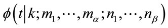 denote the conditional pgf of
  at the state
 where t is the parameter of the pgf’s. If a pgf is expanded in a standard power series in t, say
  , the coefficient
  equals the probability that at least
  frequency quotas and at least
  run quotas will be reached in n steps given that the experiment is currently at the state
  (see the Remark on page 464 in [12]). Therefore, the set of coefficients of the power series of
  gives exactly the probability distribution of the waiting time random variable
  that we wish to solve for.
The system of equations for the pgf’s of Model I comes from Equations (2) and (3) with the boundary conditions in (4) applied. Equations (2) and (3) are based on the well-known total probability formula and the boundary conditions (4) simply mean that a pgf is constant when at least  frequency quotas and at least
  run quotas are satisfied.
Beginning with the initial state we have
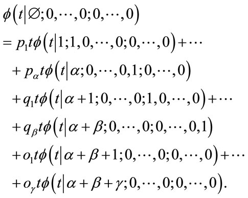 (2)
(2)
To develop a similar equation for the other incomplete states, observe that the count in a run cell is  if and only if both the cell is incomplete and the current outcome is not in that run cell. Observe also, from our earlier conventions, that no cell can have a count that exceeds its quota. Let
  be any non-initial incomplete state. Bearing in mind our above observations, for
 , define
 , and for
 , define
 , and define
  if
if  (the
(the  -th run cell is complete) and
  otherwise. We then have
 (3)
(3)
The boundary conditions which correspond to constant pgf’s are defined by
 (4)
(4)
if  is a complete state.
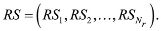
Let  be the total number of non-constant pgf’s of Model I (or the total number of equations in (2) and (3)). We will see in Section 3.3 how to calculate the value of N by (17). Let
  be the N-dimensional vector of the N non-constant pgf’s arranged in a prescribed order with
  as its first entry. Then the system of equations in (2) and (3) with the boundary conditions (4) applied can be written as
 (5)
(5)
where  is a constant matrix whose nonzero entries are the initial or transition cell probabilities (coefficients of the non-constant pgf’s) and
  is a constant vector made up from sums of cell probabilities (from the coefficients of the constant pgf’s).
It is well-known (e.g., Theorem 3.4.1 in [13]) that
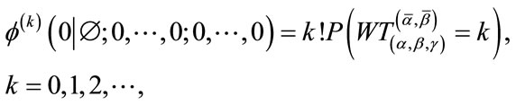 (6)
(6)
where the left-hand side is the k-th derivative of  at
at . Note that
 . By repeatedly taking derivatives in (5), we have

and thus
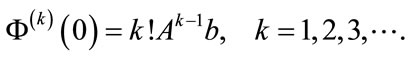 (7)
(7)
Since the pgf  is the first entry of the vector
 , by (6) and (7),
 (8)
(8)
Instead of obtaining symbolically the pgf of  , our algorithm uses the simple formula (8) to calculate the exact distribution of the waiting time variable
 . Therefore, the primary focus of our algorithm is to efficiently generate A and b. The details of how we generate A and b will be discussed in Section 3.
Since the matrix A is very sparse with each row having no more than  nonzero entries, the calculation of Ab involves no more than
  multiplications of real numbers. Since
  can be calculated from
  and
and  equals the first component of
 , the calculation of
 for all
(i.e., ) involves no more than
 multiplications of real numbers. By the nature of the problem, it can be shown that the spectral radius
  of the matrix
  is less than 1 which ensures the stability of calculating
 ,
, .
.
3. Generating A and b for Model I
In this section we will discuss how to efficiently generate the matrix A and the vector b in (5). To do this, we will generate and order the initial state  and all incomplete states of Model I of the form
  in (1) which correspond to the non-constant pgf’s at the left-hand sides of the equations in (2) and (3). (Recall that
  for
for ,
,  for
for , and the current event occurs in the k-th cell for some k,
 .) Our process will first generate all necessary arrangements
 , called frequency states, and all necessary arrangements
 , called run states, for the states in (1). Then the frequency states, run states, and possible values of k will be combined to form all incomplete states of Model I.
3.1. Generating Frequency States
The efficiency of our algorithm ultimately depends on its ability to identify the element in  in (5) that corresponds to each state. This efficiency is facilitated by the ordering of the elements in
 . In this section we will generate and order all the frequency states
  needed to construct the states in Model I.
The frequency states are first grouped into disjoint sets whose elements have in common precisely the same complete cells. Each set corresponds to exactly one binary base vector  in which if
  is a frequency state in the set, then
  if
if  (a complete cell) and
  otherwise.
To generate all the frequency states, we first generate all the base vectors necessary to form a one-to-one correspondence between the base vectors and the sets of frequency states. By the nature of Model I, once the goal of reaching  frequency quotas has been achieved, the actual subsequent counts become irrelevant in the frequency cells. All frequency states containing at least
  complete cells are thus reduced to a single frequency state representing “at least
  frequency quotas reached”. For simplicity, we use
  to denote this frequency state and we associate it with the base vector
 . Thus, only the base vectors which have less than
  1’s and the base vector
  are needed for Model I and there are

such base vectors.
We now order the base vectors, followed by an ordering of the frequency states associated with each base vector. The base vectors are grouped according to their number of 1’s. The groups themselves are then numbered and arranged in ascending order according to the number of 1’s present in each of the base vectors within the groups. The base vectors within each group are then arranged by the lexicographic order. For example, from the leftmost column of Example 1 in Section 3.2 with ,
,
 (only the zero vector),
 in this order, and
 . As a second example, for
  and
and ,
,  2 contains
  base vectors which contain exactly two 1’s. The six base vectors in
  2 have the lexicographic order
 ,
,  ,
,  ,
,  ,
,  , and
, and . Let
. Let  be the vector containing all the necessary base vectors of the frequency states, arranged in the order just described. Standard back-tracking techniques are used to generate
 .
.
We now generate and order the frequency states. Let  be a given base vector,
 . Let
. Let  be the set of all frequency states associated with
 . Note that the frequency states
  in
in  all satisfy
  if
if  and
and  if
if . We order these frequency states by the lexicographic order of their values
  for which
  (and thus the complete cells with
  have no role in the lexicographic order). Standard back-tracking techniques are used to generate all frequency states in
  in the lexicographic order just described. In the same way, we generate all the frequency states of Model I by repeating this generating process as we proceed through
  sequentially to each base vector in
 . Let
. Let  be the vector of all frequency states arranged in the order in which they were generated.
As an example of our ordering of the frequency states, see the “ ” column of Example 1 in Section 3.2.
Let ,
,  , with not all
 . The local position of a given frequency state
  in
in  can be calculated by
 (9)
(9)
where  is the largest index with
 . There is a total of
  frequency states in
 .
.
Similarly, the vector  of all frequency states contains a total of
frequency states, where we adopt the convention that
 when
when  (which corresponds to the single frequency state
 ). Thus,
 (10)
(10)
For any frequency state , its global position in the vector
  can be calculated by
 (11)
(11)
where  is the base vector associated with
 ,
,  means that the base vector
  precedes
  in the vector
 , and
, and  is the largest index with
 . The second part of this formula is from (9). The frequency state
  is naturally at the last position
  in
in .
.
Our ordering of the frequency states and the validity of Equations (9) and (11) are illustrated in the four leftmost columns of Example 1 in Section 3.2.
3.2. Generating Run States
All necessary run states of Model I can be generated and ordered similarly to the frequency states. For run states
 , base vectors
  are defined by
 if
if  (a complete cell) and
  otherwise. Thus, each base vector corresponds to a set of run states which have in common precisely the same complete run cells. Once
  run cells have reached their given quotas, all subsequent run states are reduced to one single state representing “at least
  run quotas reached”.
This run state, denoted by , is associated with the base vector
 . Thus, there are

base vectors needed to generate the run states of Model I. Let  be the vector containing these base vectors arranged in the same manner as the base vectors in Section 3.1, i.e. they are collected into groups which are arranged in ascending order of their number of 1’s, and then lexicographically ordered within their group.
To facilitate the description of our ordering of the run states, we make the following definitions:
Definition 3: Let  be a given run state. The
  -th run cell for the state
  is called active if its current run count
  satisfies
 ; otherwise, the run cell is inactive (
 or
or ). If
). If  contains an active run cell,
  is an active run state. Otherwise,
  is inactive.
Let  be a given base vector,
  and let
  be the set of run states
  associated with
 . Note that since no more than one run can be in progress at any one time, exactly one run cell is active in an active run state. Also, recall that once a run cell becomes complete (has reached its quota) its run count is fixed at its quota value. Thus, the only inactive run state in
  is given by
  if
if  and
and  if
if . All other run states in
  are active (with one active cell). The run states in
  are arranged in the lexicographic order of all the values
  for all the values of j of the incomplete run cells (and thus the complete run cells with
  have no role in the lexicographic order). Note that the first run state in this arrangement is the inactive run state in
 . For any given active run state
  in
in , its local position in
  can be calculated by
 (12)
(12)
where  is the index of the active run cell. There is a total of
  run states in
 . Standard back-tracking techniques are used to generate all run states in
  in the lexicographic order described above.
In the same way as in Section 3.1, we generate all the run states of Model I by repeating the above generating process as we proceed through  sequentially to each base vector in
 . Let
. Let  be the vector of all run states arranged in the order in which they are generated.
It can be verified that  contains a total of
run states. These are the run states needed for generating all the states of Model I. We have
 (13)
(13)
Note that for the last run state in ,
,  associated with
 , the second sum in the formula above for
  is zero vacuously. It can be verified that for any run state
 , its global position in
 can be calculated by
 (14)
(14)
if  is inactive, or
 (15)
(15)
if  is active, where
  is the base base vector associated with
 ,
,  means that the base vector
  precedes
  in the vector
 , and
, and  is the index of the active run cell in
 . The second part of the sum in (15) is from
(12).
Our ordering for both frequency and run states and the validity of the Equations (9), (11), (12), (14), and (15) to identify their positions in  and
and  are illustrated in Example 1 below.
Example 1: Let ,
,  ,
,  ,
,  , and
, and . The results discussed in Sections 3.1 and 3.2 can be summarized in the following table:
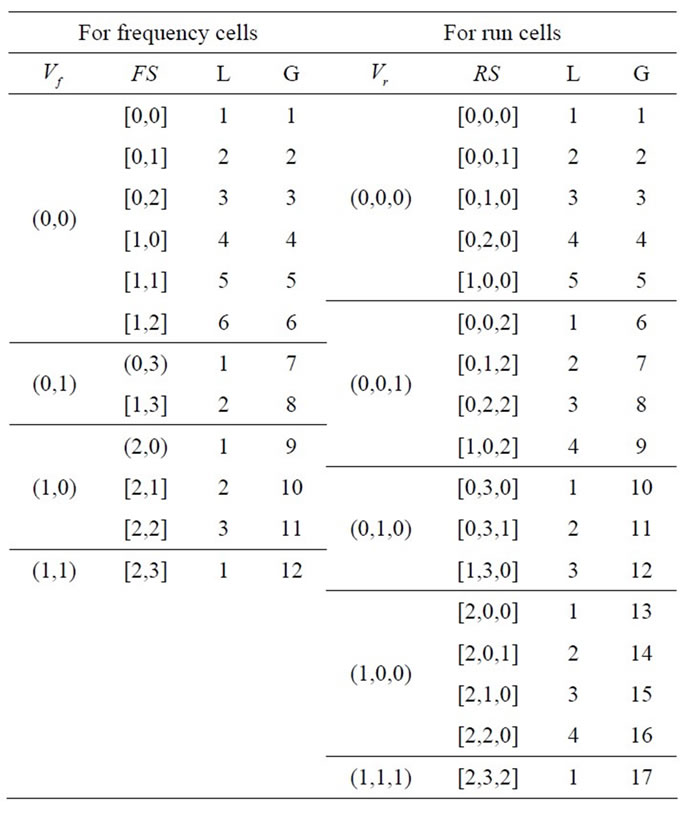
where columns “ ” and “
 ” contain the necessary base vectors for the frequency states in column “
 ” and the run states in column “
 ” respectively, the values in the columns “L” and “G” are the local positions (within the set of frequency or run states associated with the same base vector) and the global positions in
  or
or  of the corresponding frequency states or run states according to the formulas (9), (11), (12), (14), and (15).
For example, consider the run state  in Example 1. Its local position in the group associated with the base vector
  is 3. The combined count from the base vector groups
 ,
,  , and
, and  that precede the base vector group
  is 12. Thus, the global position of the run state
  in vector
  is
is . Note that the run state
  represents “at least
  run quotas reached” and thus the run base vector
  also represents the base vectors
 , and
, and .
.
3.3. Generating All States for Model I
A given frequency state  in (10) and a given run state
  in (13) can be combined to form a group of states of Model I of the form
 (16)
(16)
as in (1), where the current outcome occurs in the  -th cell for some
 ,
, . However, we will see that only a subset of values of
  taken from
  are possible in (16). For the fixed pair
 , let
, let  be the number of states in the group (16), i.e. the number of possible values of k. Let
  be the number of nonzero entries in
  and
and  be the number of complete cells in
 . If
. If  is an active run state,
  since the current outcome must be in the active run cell of
 , allowing only one value for
  in (16). If
  is inactive, the current outcome can occur in any nonzero frequency cell in
 , any complete run cell in
 , or any slack cell. Therefore, if
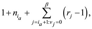
  is inactive, (16) represents a group of
 different states of Model I. We arrange the states in this group in ascending order of the values of k.
In addition to the initial state , we generate all other incomplete states of Model I by for
for 
generate states in (16) and arrange them in ascending order of the values of k end end but we exclude the combining of the frequency state
 and the run state
which corresponds to the complete state “at least  frequency quotas reached and at least
  run quotas reached”. The complete state corresponds to the constant pgf in (4) and are not part of the vector
  in (5).
Let  be the vector of all incomplete states of Model I arranged in the order they are generated above but preceded by the initial state
 as its first entry. Note that the initial state is the only state with
  since it has no current outcome. The initial state is immediately followed in
  by the group of states
  for
for
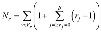
 . The total number of incomplete states for Model I is given by
 (17)
(17)
where the leading 1 corresponds to the initial state.
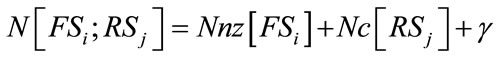
For any given state , let
, let  be the position of
  in the vector
  determined by (11) with the exception that
  if
if  ; let
; let  be the position of
  in the vector
  determined by (14) or (15); and let
  be the local position of
  , by ascending order on
 , in the group (16). The position of
  in the vector
  can be determined by
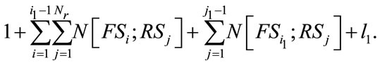 (18)
(18)
This formula is extremely useful when we generate the matrix A and the vector b.
3.4. Generating A and b
The matrix A and the vector b in (5) are initialized to zero. For each non-initial state  (
( ) in
) in
 , say
, say , the
, the
 -th row of A and element
  of b will be determined as follows: From the equation for
 in (3), if
 is a constant pgf according to the boundary conditions (4), then the value of
  is increased by
 ; otherwise
  where j is the position of the state
  in S as determined by (18). All other pgf’s on the right-hand side of (3) are then similarly processed to complete the
  -th row of A and
 . If more than one constant pgf is present on the right-hand side of (3),
  equals the sum of the probabilities of the cells corresponding to the constant pgf’s. Similarly, the first row of A and
  are determined from (2). The matrix A is stored in sparse matrix format for our computer program (e.g., Section 3.4 of [14]).
Remark 2: The states used in our algorithm are sufficient and necessary for solving the general Model I. For special cases (e.g., independent multinomial trials) certain groups of states in our algorithm can be reduced to a single state, further enhancing the efficiency of the algorithm.
4. Numerical Results
Our computer program for Model I is in C++ and is based on the methods discussed in Sections 2 and 3 for calculating the distribution, expectation, and standard deviation of the waiting time variable . Similar computer program for Model II is also developed. The programs have been successfully implemented and tested with various combinations of the parameters
 ,
,  ,
,  ,
,  ,
,  ,
,  and various probabilities. Monte Carlo simulation algorithms for both models were also developed for comparison to the pgf method.
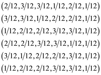
Example 2: Consider tossing one fair die initially. In every subsequent trial, we toss one of six unfair dice labeled 1 through 6. The die which is selected for the next trial matches the count on the face of the die from the current trial. Suppose we are looking for frequency quotas of 20 and 21 for faces 1 and 2, run quotas of 3 and 4 for faces 2 and 3, and faces 5 and 6 are considered slack cells. The initial cell probabilities (tossing a fair die) are  and the transition cell probabilities (tossing one of six unfair dice) are
In Example 2 . For the waiting time variables
  and
and , Table 1 lists the expectations (E), standard deviations (sd), sizes of the matrix A (N), and computation times (CPU, “m” stands for minutes and “s” for seconds) produced by the pgf method and those produced by the Monte Carlo method with 1,000,000 simulations for each possible combination of
  and each possible value of
 . The numerical values are rounded to two digits after the decimal point. The algorithm for the pgf method was terminated when, say for Model I, the condition
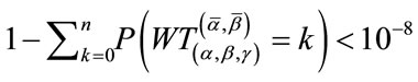 was satisfied for some
  since
since  is much smaller than
 for
for . Computation of the results was carried out on a 3.6 GHz Intel Xeon Pentium IV with 2 Gb memory running RedHat Enterprise Linux operating system.
The case  for Model I and the case
  for Model II are mathematically identical which is reflected in the results of the pgf method in
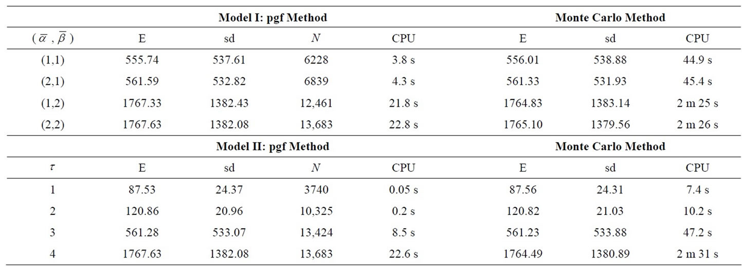
Table 1. Expectations and standard deviations for example 2.
Table 1. Note that the sizes N of the A matrices are quite large in the pgf method, but the matrices are extremely sparse. For example, the size of the matrix A is  for the parameter
  of Model II in the table. A dense matrix with this size is already too large to be handled by the computer used for the calculation in this section. But, by utilizing the sparsity of the matrices, our algorithm can efficiently solve the problem within 23 seconds and our algorithm is more than six times faster than the Monte Carlo Method. Moreover, our algorithms obtain their results by direct solution rather than by estimation based on simulations. To our knowledge, such direct solution methods were not previously available for the general Model I or Model II. The results demonstrate that our algorithms are efficient compared to the Monte Carlo simulation method.
REFERENCES
- N. Balakrishnan and M. V. Koutras, “Runs and Scans with Applications,” John Wiley & Sons, New York, 2002.
- J. C. Fu and W. Y. Lou, “Distribution Theory of Runs and Patterns and its Applications,” World Scientific Publisher, Singapore City, 2003.
- A. P. Godbole and S. G. Papastavridis, “Runs and Patterns in Probability: Selected Papers,” Kluwer, Dordrecht, 1994. doi:10.1007/978-1-4613-3635-8
- S. Aki and K. Hirano, “Sooner and Later Waiting Time Problems for Runs in Markov Dependent Bivariate Trials,” Annals of the Institute of Statistical Mathematics, Vol. 51, No. 1, 1999, pp. 17-29. doi:10.1023/A:1003874900507
- K. Balasubramanian, R. Viveros and N. Balakrishnan, “Sooner and Later Waiting Time Problems for Markovian Bernoulli Trials,” Statistics & Probability Letters, Vol. 18, No. 2, 1993, pp. 153-161. doi:10.1016/0167-7152(93)90184-K
- Q. Han and S. Aki, “Waiting Time Problems in a TwoState Markov Chain,” Annals of the Institute of Statistical Mathematics, Vol. 52, No. 4, 2000, pp. 778-789. doi:10.1023/A:1017537629251
- N. Kolev and L. Minkova, “Run and Frequency Quotas in a Multi-State Markov Chain,” Communications in Statistics—Theory and Methods, Vol. 28, No. 9, 1999, pp. 2223-2233. doi:10.1080/03610929908832417
- K. D. Ling and T. Y. Low, “On the Soonest and Latest Waiting Time Distributions: Succession Quotas,” Communications in Statistics—Theory and Methods, Vol. 22, No. 8, 1993, pp. 2207-2221. doi:10.1080/03610929308831143
- M. Sobel and M. Ebneshahrashoob, “Quota Sampling for Multinomial via Dirichlet,” Journal of Statistical Planning and Inference, Vol. 33, No. 2, 1992, pp. 157-164. doi:10.1016/0378-3758(92)90063-X
- M. Ebneshahrashoob, T. Gao and M. Sobel, “Double Window Acceptance Sampling,” Naval Research Logistics (NRL), Vol. 51, No. 2, 2004, pp. 297-306. doi:10.1002/nav.10119
- M. Ebneshahrashoob, T. Gao and M. Sobel, “Sequential Window Problems,” Sequential Analysis: Design Methods and Applications, Vol. 24, No. 2, 2005, pp. 159-175. doi:10.1081/SQA-200056194
- M. Ebneshahrashoob, T. Gao and M. Wu, “An Efficient Algorithm for Exact Distribution of Scan Statistics,” Methodology and Computing in Applied Probability, Vol. 7, No. 4, 2005, pp. 459-471. doi:10.1007/s11009-005-5003-0
- M. J. Evans and J. S. Rosenthal, “Probability and Statistics, the Science of Uncertainty,” W. H. Freeman and Company, New York, 2004.
- Y. Saad, “Iterative Methods for Sparse Linear Systems,” SIAM: Society for Industrial and Applied Mathematics, Philadelphia, 2003. doi:10.1137/1.9780898718003
NOTES
*Corresponding author.