Applied Mathematics
Vol. 3 No. 7 (2012) , Article ID: 19884 , 7 pages DOI:10.4236/am.2012.37117
Monty Hall Problem and the Principle of Equal Probability in Measurement Theory
Department of Mathematics, Faculty of Science and Technology, Keio University, Yokohama, Japan
Email: ishikawa@math.keio.ac.jp
Received April 28, 2012; revised May 28, 2012; accepted June 5, 2012
Keywords: Linguistic Interpretation; Quantum and Classical Measurement Theory; Philosophy of Statistics; Fisher Maximum Likelihood Method; Bayes’ Theorem
ABSTRACT
In this paper, we study the principle of equal probability (i.e., unless we have sufficient reason to regard one possible case as more probable than another, we treat them as equally probable) in measurement theory (i.e., the theory of quantum mechanical world view), which is characterized as the linguistic turn of quantum mechanics with the Copenhagen interpretation. This turn from physics to language does not only realize the remarkable extension of quantum mechanics but also establish the method of science. Our study will be executed in the easy example of the Monty Hall problem. Although our argument is simple, we believe that it is worth pointing out the fact that the principle of equal probability can be, for the first time, clarified in measurement theory (based on the dualism) and not the conventional statistics (based on Kolmogorov’s probability theory).
1. Introduction
1.1. Monty Hall Problem
The Monty Hall problem is well-known and elementary. Also it is famous as the problem in which even great mathematician P. Erdös made a mistake (cf. [1]). The Monty Hall problem is as follows:
Problem 1 [Monty Hall problem 1]. You are on a game show and you are given the choice of three doors. Behind one door is a car, and behind the other two are goats. You choose, say, door 1, and the host, who knows where the car is, opens another door, behind which is a goat. For example, the host says that ( ) the door 3 has a goat.
And further, He now gives you the choice of sticking with door 1 or switching to door 2? What should you do?
In the framework of measurement theory [2-12], we shall present two answers of this problem in Sections 3.1 and 4.2. Although this problem seems elementary, we assert that the complete understanding of the Monty Hall problem can not be acquired within Kolmogorov’s probability theory [13] but measurement theory (based on the dualism).
1.2. Overview: Measurement Theory
As emphasized in refs. [7,8], measurement theory (or in short, MT) is, by a linguistic turn of quantum mechanics (cf. Figure 1: ③ later), constructed as the scientific theory formulated in a certain C*-algebra A (i.e., a norm closed subalgebra in the operator algebra  composed of all bounded operators on a Hilbert space H, cf. [14,15]). MT is composed of two theories (i.e., pure measurement theory (or, in short, PMT] and statistical measurement theory (or, in short, SMT). That is, it has the following structure:
(A) MT (measurement theory)

where Axiom 2 is common in PMT and SMT. For completeness, note that measurement theory (A) (i.e., (A1) and (A2)) is not physics but a kind of language based on “the (quantum) mechanical world view”. As seen in [9], note that MT gives a foundation to statistics. That is, roughly speaking(B) it may be understandable to consider that PMT and
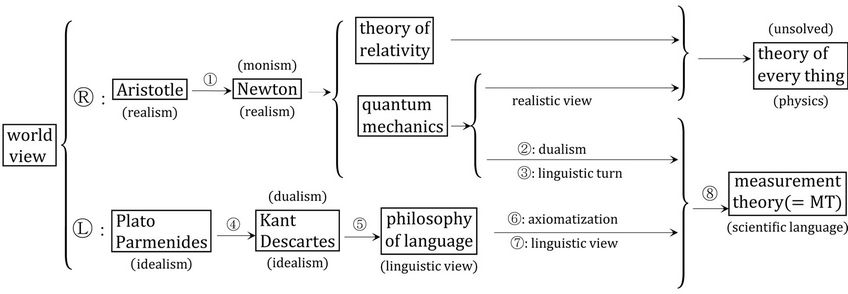
Figure 1. The development of the world views from our standing point. For the explanation of (①-⑧), see [8,10].
SMT is related to Fisher’s statistics and Bayesian statistics respectively.
Also, for the position of MT in science, see Figure 1, which was precisely explained in [8,10].
When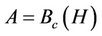 , the C*-algebra composed of all compact operators on a Hilbert space H, the (A) is called quantum measurement theory (or, quantum system theory), which can be regarded as the linguistic aspect of quantum mechanics. Also, when A is commutative (that is, when A is characterized by
 , the C*-algebra composed of all continuous complex-valued functions vanishing at infinity on a locally compact Hausdorff space
  (cf. [16])), the (A) is called classical measurement theory. Thus, we have the following classification:
(C)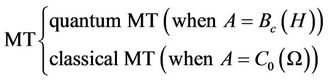
The purpose of this paper is to clarify the Monty Hall problem in the classical PMT and classical SMT.
2. Classical Measurement Theory (Axioms and Interpretation)
2.1. Mathematical Preparations
Since our concern is the Monty Hall problem, we devote ourselves to classical MT in (C). Throughout this paper, we assume that  is a compact Hausdorff space. Thus, we can put
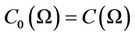 , which is defined by a Banach space (or precisely, a commutative C*-algebra) composed of all continuous complex-valued functions on a compact Hausdorff space
 , where its norm
  is defined by
 . Let
. Let  be the dual Banach space of
 . That is,
  is a continuous linear functional on
 , and the norm
  is defined by
  such that
 . The bi-linear functional
  is also denoted by
 , or in short
 .
.
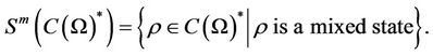
Define the mixed state  such that
  and
and  for all
  such that
 . And put
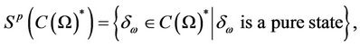
Also, for each , define the pure state
 such that
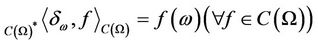 . And put
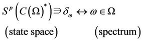
which is called a state space. Note, by the Riesz theorem (cf. [16]), that  is a signed measure on
  and
and 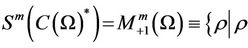 is a measure on
  such that
 . Also, it is clear that
  is a point measure at
 , where
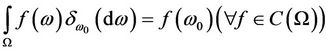 . This implies that the state space
  can be also identified with
  (called a spectrum space or simply, spectrum) such as
 (1)
(1)
Also, note that  is unital, i.e., it has the identity I (or precisely,
 ), since we assume that
  is compact.
According to the noted idea (cf. [17]) in quantum mechanics, an observable  in
in  is defined as follows:
(D1) [Field] X is a set,  , the power set of X) is a field of X, that is, “
 ”, “
”, “ ”.
”.
(D2) [Additivity] F is a mapping from  to
to  satisfying: 1): for every
 ,
,  is a non-negative element in
  such that
 , 2):
, 2):  and
and , where 0 and I is the 0-element and the identity in
  respectively. 3): for any
 ,
,  such that
 , it holds that
 .
.
For the more precise argument (such as countably additivity, etc.), see [7,9].
2.2. Classical PMT in (A1)
In this section we shall explain classical PMT in (A1).
With any system S, a commutative C*-algebra  can be associated in which the measurement theory (A) of that system can be formulated. A state of the system S is represented by an element
  and an observable is represented by an observable
  in
in . Also, the measurement of the observable O for the system S with the state
  is denoted by
  or more precisely,
  . An observer can obtain a measured value
  by the measurement
  .
.
The AxiomP 1 presented below is a kind of mathematical generalization of Born’s probabilistic interpretation of quantum mechanics. And thus, it is a statement without reality.
AxiomP 1 [Measurement]. The probability that a measured value  obtained by the measurement
  belongs to a set
  is given by
 .
.
Next, we explain Axiom 2 in (A). Let  be a tree, i.e., a partial ordered set such that “
 and
and ” implies “
 or
or ” In this paper, we assume that T is finite. Also, assume that there exists an element
 , called the root of T, such that
 holds. Put
 . The family
  is called a causal relation (due to the Heisenberg picture), if it satisfies the following conditions (E1) and (E2).
(E1) With each , a C*-algebra
  is associated.
(E2) For every , a Markov operator
  is defined (i.e.,
  ,
,  ). And it satisfies that
  holds for any
 ,
, .
.
The family of dual operators
is called a dual causal relation (due to the Schrödinger picture). When
holds for any , the causal relation is said to be deterministic.
Here, Axiom 2 in the measurement theory (A) is presented as follows:
Axiom 2 [Causality]. The causality is represented by a causal relation .
.
For the further argument (i.e., the W*-algebraic formulation) of measurement theory, see Appendix in [7].
2.3. Classical SMT in (A2)
It is usual to consider that we do not know the state  when we take a measurement
 . That is because we usually take a measurement
  in order to know the state
 . Thus, when we want to emphasize that we do not know the the state
 ,
,  is denoted by
 . Also, when we know the distribution
  of the unknown state
 , the
, the  is denoted by
 .
.
The AxiomS 1 presented below is a kind of mathematical generalization of AxiomP 1.
AxiomS 1 [Statistical measurement] The probability that a measured value  obtained by the measurement
  belongs to a set
  is given by
 .
.
Remark 1. Note that two statistical measurements ![]() and
and ![]() can not be distinguished before measurements. In this sense, we consider that, even if
can not be distinguished before measurements. In this sense, we consider that, even if , we can assume that
 (2)
(2)
2.4. Linguistic Interpretation
Next, we have to answer how to use the above axioms as follows. That is, we present the following linguistic interpretation (F) [= (F1) – (F3)], which is characterized as a kind of linguistic turn of so-called Copenhagen interpretation (cf. [7,8]). That is, we propose:
(F1) Consider the dualism composed of “observer” and “system (= measuring object)”. And therefore, “observer” and “system” must be absolutely separated.
(F2) Only one measurement is permitted. And thus, the state after a measurement is meaningless since it can not be measured any longer. Also, the causality should be assumed only in the side of system, however, a state never moves. Thus, the Heisenberg picture should be adopted.
(F3) Also, the observer does not have the space-time. Thus, the question: “When and where is a measured value obtained?” is out of measurement theory, and so on. This interpretation is, of course, common to both PMT and SMT.
Remark 2. Note that quantum mechanics has many interpretations (i.e., several Copenhagen interpretation, many worlds interpretation, statistical interpretation, etc.). On the other hand, we believe that the interpretation of measurement theory (A) is uniquely determined as in the above. This is our main reason to propose the linguistic interpretation of quantum mechanics. We believe that this uniqueness is essential to the justification of Heisenberg’s uncertainty principle (cf. [10,18]).
2.5. Preliminary Fundamental Theorems
We have the following two fundamental theorems in measurement theory:
Theorem 1 [Fisher’s maximum likelihood method (cf. [9])]. Assume that a measured value obtained by a measurement 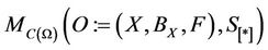 belongs to
  . Then, there is a reason to infer that the unknown state
  is equal to
 , where
  is defined by

Theorem 2 [Bayes’ method (cf. [9])]. Assume that a measured value obtained by a statistical measurement
 belongs to
 .
.
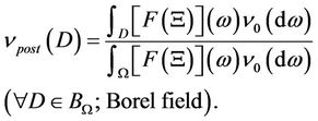
Then, there is a reason to infer that the posterior state (i.e., the mixed state after the measurement) is equal to vpost, which is defined by
The above two theorems are, of course, the most fundamental in statistics. Thus, if we believe in Figure 1, we can answer to the following problem (cf. [4,9]):
(G) What is statistics? Or, where is statistics in science? which is certainly the most essential problem in the philosophy of statistics.
3. The First Answer to Monty Hall Problem
3.1. Fisher’s Method (The First Answer)
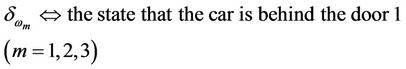
In this section, we present the first answer to Problem 1 (Monty-Hall problem) in classical PMT. Put
 with the discrete topology. Assume that each state
 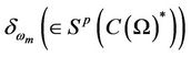 means
means
 (3)
(3)
Define the observable  in
in  such that
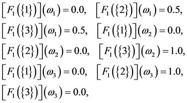 (4)
(4)
where it is also possible to assume that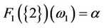 ,
, . Thus we have a measurement
 , which should be regarded as the measurement theoretical representation of the measurement that you say “door 1”. Here, we assume that
1) “measured value is obtained by the measurement ”
”  The host says “Door 1 has a goat”;
2) “measured value is obtained by the measurement ”
”  The host says “Door 1 has a goat”;
3) “measured value is obtained by the measurement ”
”  The host says “Door 1 has a goat”.
Recall that, in Problem 1, the host said “Door 3 has a goat”. This implies that you get the measured value “3”
by the measurement . Therefore, Theorem 1 (Fisher’s maximum likelihood method) says that you should pick door number 2. That is because we see that
 (5)
(5)
and thus, there is a reason to infer that . Thus, you should switch to door 2. This is the first answer to Problem 1 (the Monty-Hall problem 1).
3.2. Bayes’ Method (Answer to Modified Monty Hall Problem 2)
In the sense mentioned in Remark 3 later, the following modified Monty Hall problem (Problem 2) is completely different from Problem 1 (the Monty Hall problem 1). However, it is worth examining Problem 2 for the better understanding of Problem 3 later.
Problem 2 [Modified Monty Hall problem 2]. Suppose you are on a game show, and you are given the choice of three doors (i.e., “number 1”, “number 2”, “number 3”). Behind one door is a car, behind the others, goats. You pick a door, say number 1. Then, the host, who set a car behind a certain door, says
(#1) the car was set behind the door decided by the cast of the distorted dice. That is, the host set the car behind the k-th door (i.e., “number k”) with probability pk (or, weight such that ,
,
 ).
).
And further, the host says, for example( ) the door 3 has a goat.
He says to you, “Do you want to pick door number 2?” Is it to your advantage to switch your choice of doors?
In what follows we study this problem. Let  and
and  be as in Section 3.1. Under the hypothesis (#1), define the mixed state
  such that:
 (6)
(6)
Thus we have a statistical measurement
 . Note that
1) “measured value is obtained by the statistical measurement ”
”  The host says “Door 1 has a goat”;
2) “measured value is obtained by the statistical measurement ”
”  The host says “Door 2 has a goat”;
3) “measured value is obtained by the statistical measurement ”
”  The host says “Door 1 has a goat”.
Here, assume that, by the statistical measurement  , you obtain a measured value 3which corresponds to the fact that the host said “Door 3 has a goat”. Then, Theorem 2 (Bayes’ theorem) says that the posterior state
  is given by
 (7)
(7)
That is,
 (8)
(8)
Particularly, we see that (H) if , then it holds that
 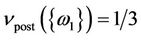 ,
, 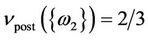 ,
, 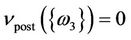 , and thus, you should pick Door 2.
Remark 3. The difference between Problem 1 and Problem 2 should be remarked. Since the (#1) in Problem 2 is the information from the host to you, Problem 1 and Problem 2 are completely different. Although the above (H) may be generally regarded as the proper answer of the Monty Hall problem, we do not admit that the (H) is proper. That is, we consider that the (H) is not the second answer to the Monty Hall problem.
4. The Second Answer to Monty Hall Problem
In this section, we shall present the second answer. However, before it, we have to prepare the principle of equal probability (i.e., unless we have sufficient reason to regard one possible case as more probable than another, we treat them as equally probable). For completeness, note that measurement theory urges us to use only Axioms 1 and 2.
4.1. The Principle of Equal Probability
Put  with the discrete topology. And consider any observable
  in
in .
.
Define the bijection  such that
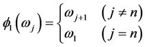
and define the observable  in
in  such that
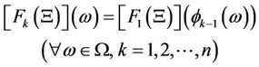
where  and
and
 .
.
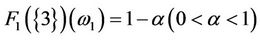
Let  be a non-negative real number such that
 .
.
(I) For example, fix a state . And, by the cast of the distorted dice, you choose an observable
  with probability pk. And further, you take a measurement
 .
.
Here, we can easily see that the probability that a measured value obtained by the measurement (I) belongs to  is given by
 (9)
(9)
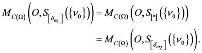
which is equal to . This implies that the measurement (I) is equivalent to a statistical measurement:
 .
.
Note that the (9) depends on the state . Thus, we can not calculate the (9) such as the (8).
However, if it holds that , we see that
  is independent of the choice of the state
 . Thus, putting
 , we see that the measurement (I) is equivalent to the statistical measurement
 , which is also equivalent to
  (from the formula (2) in Remark 1).
Thus, under the above notation, we have the following theorem.
Theorem 3 [The principle of equal probability (i.e., the equal probability of selection)]. If 
 , the measurement (I) is independent of the choice of the state
 . Hence, the (I) is equivalent to a statistical measurement
 .
.
It should be noted that the principle of equal probability is not “principle” but “theorem” in measurement theory.
Remark 4. This theorem was also discussed in [5,6], where we missed the formula (2) in Remark 1. Thus, the argument in [5,6] was too abstract. And thus, it might be regarded as ambiguous and vague. In fact, we must admit that the explanation in [5,6] is not yet accepted generally. Therefore, we recommend readers to read [5,6] after the understanding of the concrete explanation (I) in the linguistic interpretation (F). Also, note that Theorem 3 is independent of Axiom 2. And further, for the principle of equal (a priori) probabilities in equilibrium statistical mechanics, see [11], in which how to use measurement theory (and thus statistics) in statistical mechanics is explained.
4.2. The Second Answer to Monty Hall Problem (i.e., Modified Monty Hall Problem 3)
As an application of Theorem 3, we consider the following modified Monty-Hall problem:
Problem 3 [Modified Monty Hall problem 3]. Suppose you are on a game show, and you are given the choice of three doors (i.e., “number 1”, “number 2”, “number 3”). Behind one door is a car, behind the others, goats.
(#2) You choose a door by the cast of the fair dice, i.e., with probability 1/3.
According to the rule (#2), you pick a door, say number 1, and the host, who knows where the car is, opens another door, behind which is a goat. For example, the host says that
( ) the door 3 has a goat.
He says to you, “Do you want to pick door number 2?” Is it to your advantage to switch your choice of doors?
[Answer]. Consider  and O1 as in Section 3.1. Then, Theorem 3 says that the answer of Problem 3 is the same as the (H). Thus, you should pick the door 2.
Remark 5. The difference between the (#1) in Problem 2 and the (#2) in Problem 3 is clear in the dualism (F). The former is host’s selection, but the latter is your selection (i.e., observer’s selection). That is, in Problem 3, the information from host to you is only the ( ). This situation is the same as that of Problem 1. In this sense, we think that Problems 1 and 3 are similar. That is, we can conclude that Problem 1 [resp. Problem 3] is the Monty Hall problem in PMT [resp. SMT]. Also, our recent report [19] will promote a better understanding of measurement theory.
5. Conclusions
In the conventional statistics based on Kolmogorov’s probability theory, Problem 3 may be unconsciously confused with Problem 2. On the other hand, as mentioned in Remark 5, the difference between Problems 2 and 3 can be clearly described in measurement theory (based on the dualism (F)). This is the merit of measurement theory.
What we executed in this paper may be merely the translation from “ordinary language” to “scientific language”, that is,

We believe that this translation is just “the mechanical world view” or “the method of science” (at least, science in the series L of Figure 1). That is, ordinary science (at least, its basic statements) should be described in terms of measurement theory. For example, for the translation of equilibrium statistical mechanics and the Zeno’s paradoxes, see [11] and [12] respectively. Probably, we refrained from the publication of [12], if we were not sure of “MT = the method of science (or the form of scientific thinking)”.
In this paper (as well as [9]), we showed one of advantages of the measurement theoretical foundation of statistics through the examination of the Monty Hall problem. Also, recall that measurement theory possesses a great power to answer to the problem (G). However, our methodology should be tested from various points of view, because the classic statistics methodology (based on Kolmogorov’s probability theory) can be good applied in many fields. We hope that our approach will be examined from various view points.
REFERENCES
- P. Hoffman, “The Man Who Loved Only Numbers, the Story of Paul Erdös and the Search for Mathematical Truth,” Hyperion, New York, 1998,
- S. Ishikawa, “Fuzzy Inferences by Algebraic Method,” Fuzzy Sets and Systems, Vol. 87, No. 2, 1997, pp. 181-200. doi:10.1016/S0165-0114(96)00035-8
- S. Ishikawa, “A Quantum Mechanical Approach to Fuzzy Theory,” Fuzzy Sets and Systems, Vol. 90, No. 3, 1997, pp. 277-306. doi:10.1016/S0165-0114(96)00114-5
- S. Ishikawa, “Statistics in Measurements,” Fuzzy Sets and Systems, Vol. 116, No. 2, 2000, pp. 141-154. doi:10.1016/S0165-0114(98)00280-2
- S. Ishikawa, “Mathematical Foundations of Measurement Theory,” Keio University Press Inc., 2006. http://www.keio-up.co.jp/kup/mfomt/
- S. Ishikawa, “Monty Hall Problem in Unintentional Random Measurements,” Far East Journal of Dynamical Systems, Vol. 3, No. 2, 2009, pp. 165-181.
- S. Ishikawa, “A New Interpretation of Quantum Mechanics,” Journal of Quantum Information Science, Vol. 1, No. 2, 2011, pp. 35-42. doi:10.4236/jqis.2011.12005
- S. Ishikawa, “Quantum Mechanics and the Philosophy of Language: Reconsideration of Traditional Philosophies,” Journal of Quantum Information Science, Vol. 2, No. 1, 2012, pp. 2-9. doi:10.4236/jqis.2012.21002
- S. Ishikawa, “A Measurement Theoretical Foundation of Statistics,” Applied Mathematics, Vol. 3, No. 3, 2012, pp. 183-192.
- S. Ishikawa, “The Linguistic Interpretation of Quantum Mechanics,” 2012. http://arxiv.org/pdf/1204.3892.pdf
- S. Ishikawa, “Ergodic Hypothesis and Equilibrium Statistical Mechanics in the Quantum Mechanical World View,” World Journal of Mechanics, Vol. 2, No. 2, 2012, pp. 125-130. doi:10.4236/wjm.2012.22014
- S. Ishikawa, “Zeno’s Paradoxes in the Mechanical World View,” 2012. http://arxiv.org/pdf/1205.1290.pdf
- A. Kolmogorov, “Foundations of the Theory of Probability (Translation),” Chelsea Pub Co. Second Edition, New York, 1960.
- G. J. Murphy, “C*-Algebras and Operator Theory,” Academic Press, Boston, 1990.
- J. von Neumann, “Mathematical Foundations of Quantum Mechanics,” Springer Verlag, Berlin, 1932.
- K. Yosida, “Functional Analysis,” 6th Edition, SpringerVerlag, Berlin, 1980.
- E. B. Davies, “Quantum Theory of Open Systems,” Academic Press, London, 1976.
- S. Ishikawa, “Uncertainty Relation in Simultaneous Measurements for Arbitrary Observables,” Reports on Mathematical Physics, Vol. 29, No. 3, 1991, pp. 257-273. doi:10.1016/0034-4877(91)90046-P
- S. Ishikawa, “What Is Statistics? The Answer by Quantum Language,” arXiv:1207.0407v1 [physics.data-an], 2012. http://arxiv.org/abs/1207.0407v1