Journal of Environmental Protection
Vol. 4 No. 6 (2013) , Article ID: 33421 , 12 pages DOI:10.4236/jep.2013.46075
A Fair Plan to Safeguard Earth’s Climate. 3: Outlook for Global Temperature Change throughout the 21st Century
![]()
Climate Research Group, Department of Atmospheric Sciences, University of Illinois at Urbana-Champaign, Urbana, USA.
Email: schlesin@atmos.uiuc.edu
Copyright © 2013 Michael E. Schlesinger et al. This is an open access article distributed under the Creative Commons Attribution License, which permits unrestricted use, distribution, and reproduction in any medium, provided the original work is properly cited.
Received April 9th, 2013; revised May 12th, 2013; accepted June 8th, 2013
Keywords: Climate Change; Global Warming; Greenhouse-Gas Emissions; Mitigation
ABSTRACT
We apply Singular Spectrum Analysis to four datasets of observed global-mean near-surface temperature from start year to through 2012: HadCRU (to = 1850), NOAA (to = 1880), NASA (to = 1880), and JMA (to = 1891). For each dataset, SSA reveals a trend of increasing temperature and several quasi-periodic oscillations (QPOs). QPOs 1, 2 and 3 are predictable on a year-by-year basis by sine waves with periods/amplitudes of: 1) 62.4 years/0.11˚C; 2) 20.1 to 21.4 years/0.04˚C to 0.05˚C; and 3) 9.1 to 9.2 years/0.03˚C to 0.04˚C. The remainder of the natural variability is not predictable on a year-by-year basis. We represent this noise by its 90 percent confidence interval. We combine the predictable and unpredictable natural variability with the temperature changes caused by the 11-year solar cycle and humanity, the latter for both the Reference and Revised-Fair-Plan scenarios for future emissions of greenhouse gases. The resulting temperature departures show that we have moved from the first phase of learning—Ignorance—through the second phase—Uncertainty—and are now entering the third phase—Resolution—when the human-caused signal is much larger than the natural variability. Accordingly, it is now time to transition to the post-fossil-fuel age by phasing out fossil-fuel emissions from 2020 through 2100.
1. Introduction
In our year-2000 “Causes of Global Temperature Changes During the 19th and 20th Centuries” paper we concluded: “Accordingly, it is prudent not to expect year-after-year warming in the near future and, in so doing, diminish concern about global warming should global cooling instead manifest itself again (as it did from 1944 to 1976)” [1] (hereafter Causes 1). This caution notwithstanding, some climate skeptics have concluded that there is no human-caused global warming because during the time period 1998 to 2008, there was no increase in the globalmean near-surface temperature [2]. In our 2012 paper, “Causes of the Warming Observed Since the 19th Century” [3] (hereafter Causes 2), we showed that the absence of warming during 1998-2008 was the result of natural cooling counteracting the human-caused warming. Recently Andy Revkin, author of the Dot Earth blog on the NY Times website [4], emailed us “… but if the “pause” (in global warming) persists through 2017 or longer (absent some obvious push like eruptions), that could raise questions (about the reality of human-caused warming) [5].”
Accordingly, in this paper we examine the issue of future naturally occurring variability in the Earth’s climate system in comparison with human-caused global warming. To do so we will analyze the observed changes in Earth’s global-mean near-surface temperature from 1850 to 2012 to project future temperature changes through 2100. We will combine this natural variability, both predictable year-by-year and unpredictable year-by-year, with the human-caused changes in global-mean nearsurface temperature for the Reference and Mitigation scenarios of our two 2012 papers, “A Fair Plan to Safeguard Earth’s Climate [6] (hereafter FP1) and a “Revised Fair Plan to Safeguard Earth’s Climate” [7] (hereafter FP2). In so doing we shall show that the time when natural variability in the Earth’s climate system could counterbalance human-caused global warming is coming to an end because humanity has now become the dominant shaper of Earth’s future climate. We shall thereby show, yet again as we did in FP2, that unless humanity reduces its emission of greenhouse gases to zero from 2020 through 2100, the rise in global-mean near-surface temperature will exceed the 2˚C (3.6˚F) limit adopted by the UN Framework Convention on Climate Change “to prevent dangerous anthropogenic interference with the climate system” [8,9].
2. Analysis of the Observed Changes in Global-Mean Near-Surface Temperature, 1850 through 2012
The observed changes in global-mean near-surface temperature are due to two factors, one external to the climate system, and the other internal thereto. The external factors influence climate but are not influenced by climate. These include variations in solar irradiance and volcanoes. The internal factors influence climate and are influenced by climate. These include the interactions among the components of the climate system—the atmosphere, ocean, cryosphere, geosphere and biosphere— and human changes to the climate system.
In 1994, we published our first paper analyzing the observed changes in global-mean near-surface temperature, “An Oscillation in the Global Climate System of Period 65 - 70 Years” [10]. Therein we used a then recently developed method of spectral analysis called Singular Spectrum Analysis (SSA). In SSA the mathematical structures (basis functions) onto which the observed temperature departures from the 1961-1990 mean temperature are projected, are not prescribed (usually trigonometric functions) but instead are determined by the observed temperatures themselves. Doing this allows SSA to find statistically significant structures in the data that ordinary Fourier analysis cannot. Because of this we discovered a 65 - 70 year oscillation in the global-mean near-surface temperature record that was due to an oscillation in the near-surface temperature over the North Atlantic Ocean. This oscillation has come to be known as the Atlantic Multidecadal Oscillation (AMO). It is this AMO that caused the early twentieth century warming (1904 to 1944) and subsequent mid-twentieth century cooling (1944 to 1976) [1,3,10]. It is the latter that caused us to write the cautionary warning stated in the Introduction.
2.1. Observed Global-Mean Near-Surface Temperature Data
We shall not elaborate the mathematics of SSA here, as we have thoroughly done so in our earlier papers [1,3, 10]. We do note however that we no longer use our Simple Climate Model [1,10,11] to detrend the observed record of global-mean near-surface temperatures before applying SSA, as we did in our 1994 and 2000 (Causes 1) papers [1,10]. Rather, we determine this trend by SSA itself and, thereby, do not impose a model on the data before applying SSA thereto. We first did this in our Causes 2 paper [3]. In that paper we analyzed the observed near-surface temperature records of the four groups that annually provide these data, namely: 1) the Hadley Centre-Climate Research Unit (HadCRU) located in the United Kingdom, with data starting in 1850 [12]; 2) the National Climate Data Center of the US National Oceanographic and Atmospheric Administration (NOAA) located in Asheville, North Carolina, with data starting in 1880 [13]; 3) the Goddard Institute of Space Studies of the US National Aeronautics and Space Administration (NASA) located in New York City, with data starting in 1880 [14]; and 4) the Japanese Meteorological Agency (JMA) located in Tsukuba, Japan, with data starting in 1891 [15,16]. We shall see that the start dates of the NOAA, NASA and JMA datasets are too late to correctly determine the structure of the AMO, the most important variation in the four datasets. In our Causes 2 paper we analyzed these four observational datasets through 2010. Here we add two more years of data—2011 and 2012.
Figure 1 shows the four observed global-mean nearsurface temperature departures from the 1961-1990 average temperature (black line), together with their SSAdetermined trend (red line). As we showed in our Causes 2 paper, the global-warming trend determined by SSA is caused by humanity through: 1) the release of carbon dioxide (CO2) by the burning of fossil fuels: coal, natural gas and oil; 2) the release of methane (CH4) by flatulent livestock animals in animal husbandry, coal mining and land fills; 3) nitrogen dioxide (N2O) by the use of nitrogen-rich fertilizer in agriculture to replenish the nitrogen taken out of the soil and fixed in agricultural biomass; and 4) the release of human-made chloroflurocarbons (CFCs) used as spray propellants and refrigerants. It is evident from Figure 1 that there is a rich variability in the global-mean near-surface temperature in addition to the human-caused global warming from the mid 19th century to the present.
2.2. Quasi-Periodic Oscillations in the Observed Global-Mean Near-Surface Temperature Data
Figure 2 shows the SSA analysis of the natural variability. Shown therein are the first four Quasi-periodic Oscillations (QPOs) revealed by SSA. These QPOs are oscillations with variable periods and amplitudes. QPO-1, shown in Figure 2(A), has a period of about 60 years and an amplitude of about 0.1˚C. This is the AMO discovered by us in 1994 [10]. The structure of QPO-1 shown by the NOAA, NASA and JMA data differs from the structure shown by the HadCRU data. We shall return to this below. QPO-2, shown in Figure 2(B), has a period of about 20 years and an amplitude of about 0.05˚C. This oscillation was found by us in our 1994 paper [10] and earlier
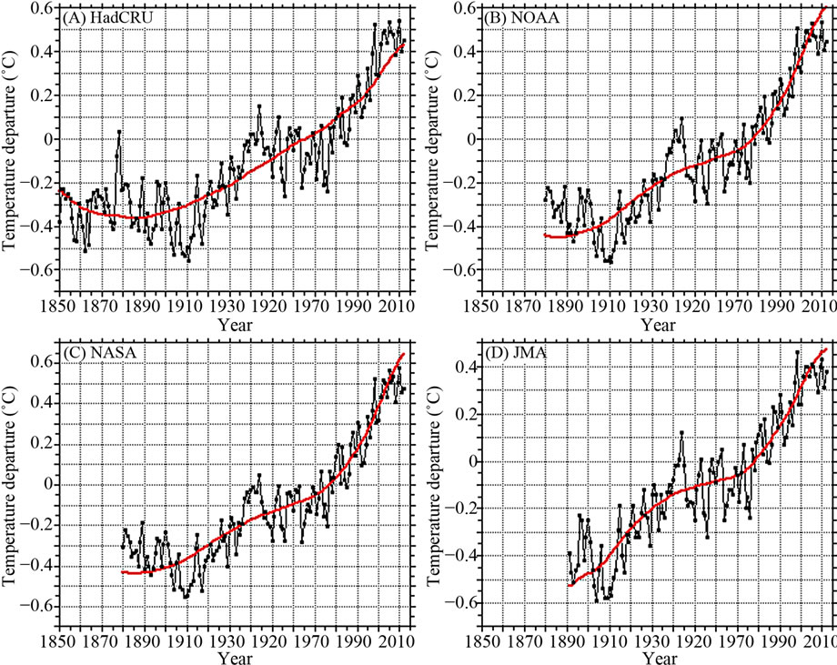
Figure 1. Observed departure of global-mean near-surface temperature from the 1961-1990 average (black line), and the trend thereof determined by singular-spectrum-analysis (red line) for: (A) HadCRU, 1850-2012; (B) NOAA, 1880-2012; (C) NASA, 1880-2012, and (D) JMA, 1891-2012.
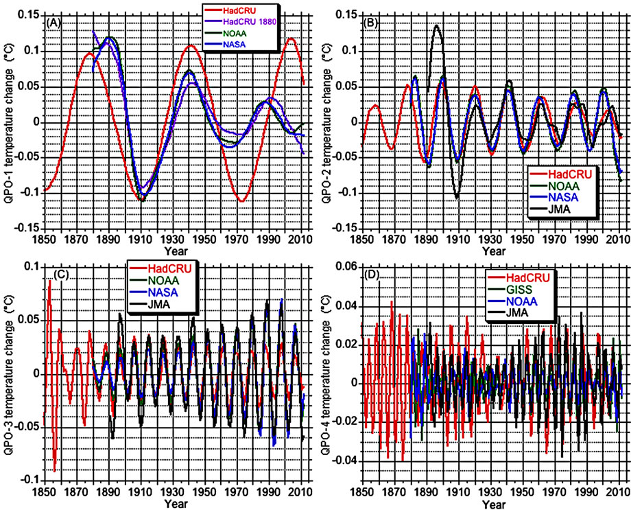
Figure 2. Quasi-periodic oscillations (QPOs) determined by singular-spectrum analysis of the HadCRU (red line), NOAA (green line), NASA (blue line) and JMA (black line) global-mean near-surface temperature departures shown in Figure 1: (A) QPO-1, (B) QPO-2, (C) QPO-3 and (D) QPO-4. The purple line in panel A shows QPO-1 obtained by SSA when the years 1850 to 1879 are excluded.
by Ghil and Vautard [17]. QPO-3, shown in Figure 2(C), has a period of about 10 years and an amplitude of about 0.05˚C. QPO-4 has an irregular period shorter than 10 years and an irregular amplitude whose average is about 0.02˚C. There are three other QPOs in the data (not shown) with even more irregular interannual periods and smaller amplitudes, as well as a stochastic (random) noise component. We will see in Section 3 that it is possible to represent QPOs 1, 2 and 3 mathematically and thus project them forward in time year by year. Alas, it is not possible to do so with QPO-4 and the higher-order QPOs. Accordingly, we shall represent their effect on the global-mean temperature, and the effect thereon by stochastic noise, by their 90 percent confidence interval.
2.2.1. Influence of Start Date on QPO-1
Figure 2 shows that when the start date of the HadCRU data is changed from 1850 to 1880, the structure of its QPO-1 is very similar to that obtained from the NOAA and NASA data that start in 1880. Accordingly we conclude that a start date of 1880 is too late to correctly characterize the structure of QPO-1. It is of interest therefore to examine when the structure of QPO-1 with start date between 1850 and 1880 agrees with the structure of QPO-1 for the start date of 1850.
Figure 3(A) shows the structure of QPO-1 for the Had-CRU temperature observations for start dates from 1850 to 1880 in 10-year intervals, and Figure 3(B) shows the Coefficient of Determination (R2) of QPO-1 for these start dates with QPO-1 for the actual start date of 1850. It is seen that for R2 to exceed 0.9, the start date must be no later than 1860. Accordingly, a record length of about 152 years is required to correctly determine the structure of QPO-1. This record length will be attained for the NOAA and NASA data in 2032, and for the JMA data in 2043. This is 19 and 30 years into the future. As this is a long time to wait to determine the structure of QPO-1 from the NOAA, NASA and JMA data, we suggest that these groups extend their temperature observations backward in time to 1850.
2.2.2. Influence of End Date on the HadCRU QPO-1
It is also of interest to examine how the structure of QPO-1 for the HadCRU temperature observations changed by the addition of the temperatures for 2011 and 2012. This is shown in Figure 3(C). The addition of two more years of data has caused both the period and the amplitude of QPO-1 to become more uniform. This is also seen in Figure 3(D) which presents the year-by-year predictable part of the HadCRU temperature observations given by QPO-1 + QPO-2 + QPO-3. This suggests that the analysis reported here should be repeated at least
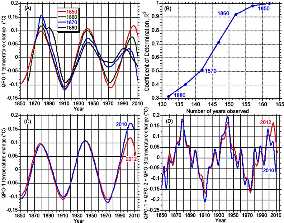
Figure 3. (A) The structure of QPO-1 obtained for the HadCRU temperature observations for starting years 1850 to 1880 in 10-year intervals; (B) The Coefficient of Determination, R2, of the structure of QPO-1 for the HadCRU temperature observations for starting years 1850 to 1880 in 5-year intervals with the 1850 structure; (C) The structure of QPO-1 for the HadCRU temperature observations for ending years of 2010 and 2012; (D) The year-by-year predictable part of the HadCRU temperature observations given by QPO-1 + QPO-2 + QPO-3.
every five years.
3. Projection of Temperature Changes from 2012 through 2100
The temperature changes due to internal factors consist of two parts: 1) a predictable part that can be projected year to year; and 2) an unpredictable part that cannot be projected year to year. QPOs 1, 2 and 3 are sufficiently regular that they can be predicted on a year-to-year basis. The higher-order QPOs and the stochastic noise cannot be predicted on a year-to-year basis. We will represent these unpredictable temperature changes by their 90- percent confidence interval—the interval between the 5th and 95th percentiles of their cumulative distribution function (CDF).
3.1. Predictable Temperature Changes
We have examined 7 methods for representing the predictable part of the natural variability: 1) the “SSA-vector” and “SSA-recurrent” methods implemented in the RSSA package [18,19] of the statistical software R [20]; 2) four auto-regressive (AR) methods: “AR-Burg”, “AROLS”, “AR-MLE” and “AR-Yule-Walker”; and 3) representation by the sine wave y(t) = C + A sin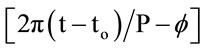 , with parameters C, A, P and f determined by the Kaleidagraph software package [21], with to being the start year of the observed temperature dataset. These methods and their evaluation are described in the Appendix. We found the sine-wave representation to be superior to the other 6 methods.
Figure 4 shows the sine-wave representations of QPOs 1, 2 and 3 from 1850 through 2100 for the HadCRU observed temperature data. The C, A, P and f parameters of these fits, and for the fits for the NOAA, NASA and JMA datasets, are presented in Table 1. Therein it is seen that the coefficient of determination between QPO-1 and its fit for the HadCRU dataset is 0.993. We use this fit for the NOAA, NASA and JMA datasets because, as discussed in Section 2.2.1, their duration is too short to correctly characterize QPO-1.
The coefficient of determination for QPO-2 is above 0.867 for the HadCRU, NOAA and NASA datasets, but is only 0.472 for the JMA dataset. In contrast, the coefficient of determination for QPO-3 is highest (0.899) for the JMA dataset and lowest (0.703) for the HadCRU dataset. Accordingly, it should be kept in mind that the combined temperature change due to QPO-1 + QPO-2 + QPO-3 is not fully predictable, but rather only quasipredictable.
In our Causes 2 paper we used our Simple Climate Model to simulate the temperature change from 1765 through 2010, ΔTSIM(t), due to solar-irradiance variations, volcanoes and humanity, the latter by the emissions of greenhouse gases and aerosol precursors, and land-use changes. In so doing we determined the climate sensitivity, ΔT2x—the change in global-mean, equilibrium nearsurface temperature due to a doubling of the pre-industrial CO2 concentration—that best reproduced the observed temperature departures δTOBS(t) from the 1961-90 mean temperature for the HadCRU, NOAA, NASA and JMA temperature observations. As shown in Table 2, this yielded ΔT2x = 1.61˚C, 1.99˚C, 1.45˚C and 2.01˚C, respectively. In so doing we converted ΔTSIM(t) to the simulated temperature departures from the 1961-1990 average temperature by
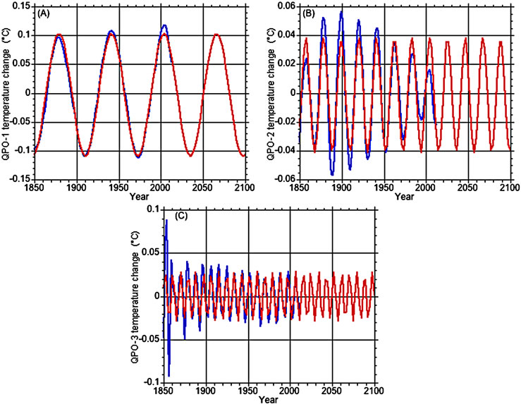
Figure 4. Sine-wave representations y(t) = C + A sin[2π(t − to)/P − f] (red line) of QPO-1 (A), QPO-2 (B) and QPO-3 (C) for the HadCRU temperature observation (blue line) shown in Figure 2.
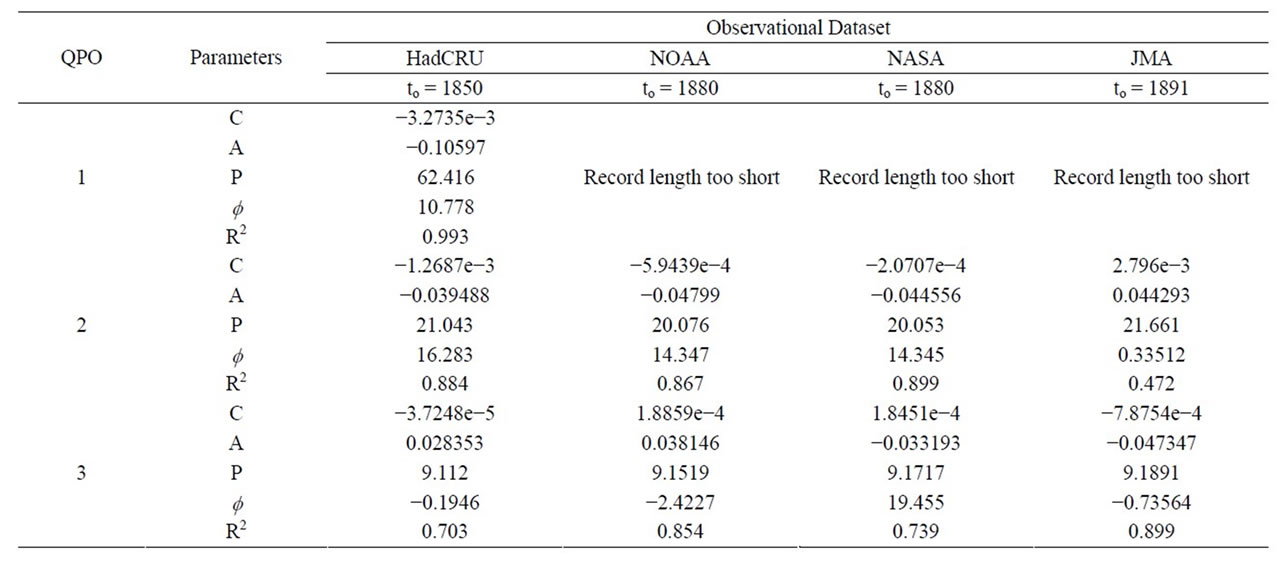
Table 1. Characteristics of the predictable natural variability. Values of the parameters of the sine-wave representations y(t) = C + A sin[2π(t − to)/P − f], and coefficients of determination (R2), for QPOs 1, 2 and 3 for the HadCRU, NOAA, NASA and JMA observed temperature datasets.
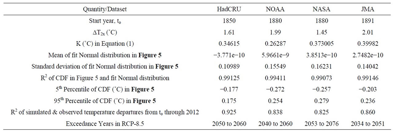
Table 2. Characteristics of the unpredictable natural variability for the HadCRU, NOAA, NASA and JMA observed temperature datasets.
 (1)
(1)
where K for each observed dataset was determined such that the average of δTSIM(t) − δTOBS(t) from starting year to through 2010 was zero, with to = 1850 for the HadCRU observations, 1880 for the NOAA and NASA observations, and 1891 for the JMA observations.
We now combine δTSIM(t) with the fit temperature changes due to QPOs 1, 2 and 3 to obtain the total predictable temperature changes from to through 2100,
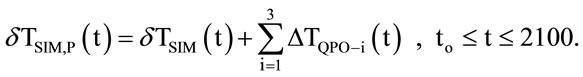 (2)
(2)
In Section 3.3 we describe the two scenarios of future greenhouse-gas emissions for which we simulated ΔTSIM(t) from to through 2100 and then converted them to the corresponding δTSIM(t) via Equation (1).
3.2. Unpredictable Temperature Changes
We define the unpredictable temperature change, δTUP(t), by
 (3)
(3)
The cumulative distribution function (CDF) for δTUP(t) is shown in Figure 5 for the four observed temperature datasets. It is seen that the CDFs are very well fit by the CDF for a Normal distribution, shown by the red line in each panel, with a coefficient of determination R2 > 0.99. Mathematically this fit is μ + σ norm(x), where μ and σ are the median and standard deviation for the Normal distribution. The characteristics of the fit Normal distributions are presented in Table 2. The median (= mean = mode) for the fit for each of the four datasets is essentially zero ˚C, showing that there is no bias in the unpre-
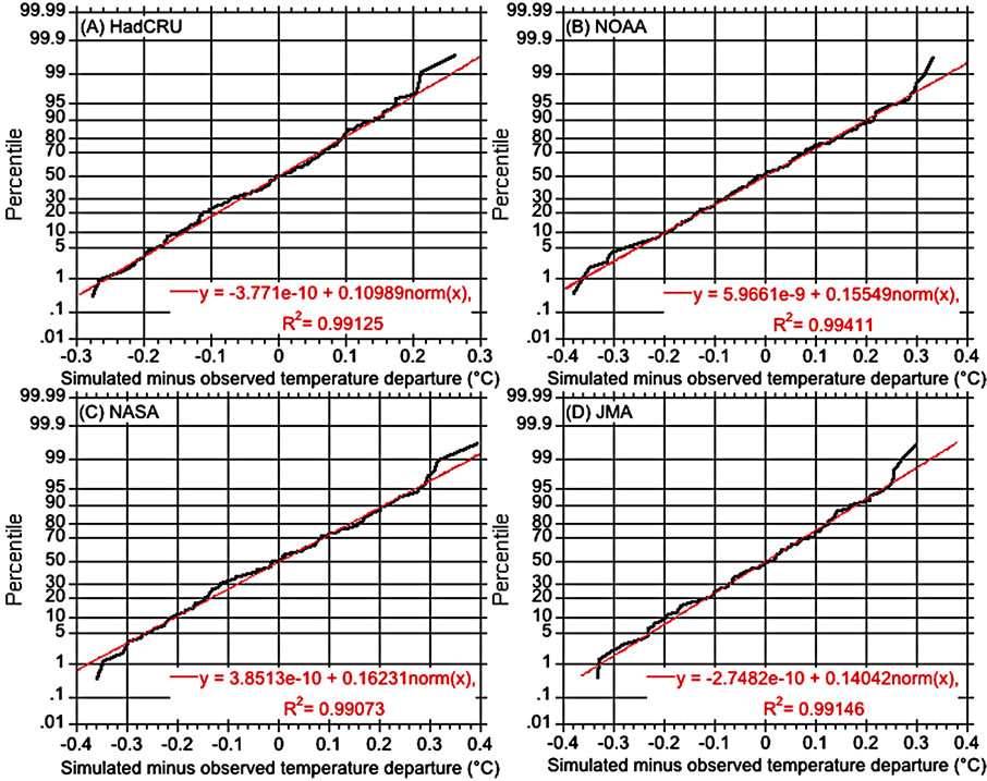
Figure 5. Cumulative distribution function (CDF) for the unpredictable temperature change, δTUP(t) = δTSIM,P(t) − δTOBS(t), to ≤ t ≤ 2012 (black curve). The fit by the normal distribution (red curve) is μ + σ norm(x), wherein μ and σ are the median (= mean = mode) and standard deviation, respectively.
dictable temperature change, δTUP(t). The standard deviation for the NOAA, NASA and JMA datasets lies between 0.140˚C and 0.162˚C. This is about 50% larger than the standard deviation for the HadCRU dataset of 0.110˚C. Undoubtedly this is because we have used QPO-1 for the HadCRU data as the QPO-1 for the NOAA, NASA and JMA data, this because, as shown in Section 2.2.1, the record length of these three datasets is too short to accurately characterize QPO-1.
The 5th and 95th percentiles of the actual CDFs, ΔT5th and ΔT95th are shown in Table 2. In Section 4 we will present δTSIM,P(t) + ΔT5th, δTSIM,P(t) and δTSIM,P(t) + ΔT95th for to ≤ t ≤ 2100 for two scenarios of future greenhouse-gas emissions. It should be noted here that while we include solar-irradiance variations in δTSIM,P(t) due to the 11-year sunspot cycle, we do not include any other solar variations, nor do we include any future volcanic eruptions, as their timing, duration and intensity cannot now be predicted.
3.3. Future Emission Scenarios
In FP1 we used our Simple Climate Model [11] to calculate the change in global-average near-surface air temperature from 1765 through year 3000 for two scenarios of the future emissions of greenhouse gases (GHGs), a Reference scenario—the Representative Concentration Pathway 8.5 scenario (RCP-8.5)—and a Mitigation scenario—the Fair Plan scenario. The latter is fair in two ways. First, it uses trade-adjusted emissions, that is, the GHG emissions incurred by country X in producing goods and services imported by country Y are considered as the GHG emissions of country Y, not country X. Second, the intensity of GHG emissions of the developed (so-called Annex B or AB) countries and developing (non-Annex B or nAB) countries were decreased differently from unity in 2015 to zero in 2065 such that: 1) the cumulative GHG emissions for AB and nAB countries were equal; and 2) the maximum increase in global-mean near-surface temperature did not exceed the 2˚C limit adopted by the United Nations Framework Convention on Climate Change “to prevent dangerous anthropogenic interference with the climate system” [8,9]. The GHG intensity decreased from unity in 2015 to zero in 2065 linearly for AB countries and more slowly at first for nAB countries, thereby allowing their continuing economic development. In FP2 we examined the effect of: 1) deferring the start year from 2015 to 2030 in 5-year increments; and 2) increasing the phase-out period from 50 years to 100 years in 10-year increments. We found that it is optimum to begin the phase-out in 2020 and complete it in 2100. Accordingly, below we present δTSIM,P(t) + ΔT5th, δTSIM,P(t) and δTSIM,P(t) + ΔT95th for to ≤ t ≤ 2100 for the RCP-8.5 and FP2 scenarios of future greenhouse-gas emissions.
4. Temperature Departures for the RCP-8.5 and FP2 Emissions Scenarios
Figure 6 presents the simulated temperature changes from 1765 through year 3000 for the Reference RCP-8.5 and FP2 Mitigation scenarios for the climate sensitivities obtained by optimizing the agreement between the simulated and observed temperature deviations from the 1961- 90 mean, the latter for the HadCRU, NOAA, NASA and JMA datasets. The results for the HadCRU, NOAA and NASA (GISS) datasets are from Figure 1(C) of FP1 and Figure 9 of FP2. The results for JMA were obtained for this paper (FP3). The UNFCCC limit of 2˚C is shown by the green line. The simulated temperature changes from to through 2012 include the human-caused contributions due to the emission of greenhouse gases and aerosol precursors, and land-use changes. They also include variations in solar irradiance due to the 11-year sunspot cycle and the Maunder Minimum therein, and volcanoes. The simulated temperature changes from 2012 through year 3000 include the human-caused contributions due to the emission of greenhouse gases and aerosol precursors for each scenario, and variations in solar irradiance due to the 11-year sunspot cycle.
Figure 6 shows that the temperature change for the RCP-8.5 scenario exceeds the UNFCCC limit starting from 2047 (JMA) to 2062 (NASA), and peaks circa 2250 with values from 4.4˚C (NASA) to 6.0˚C (JMA). The temperature change for FP2 peaks in about 2080 and ranges from 1.7˚C (NASA) to 2.3˚C (JMA). The temperature changes for JMA and NOAA slightly exceed the 2˚C UNFCCC limit from 2056 to 2130 for JMA, and
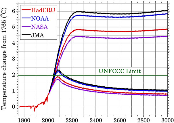
Figure 6. Simulated temperature change from 1765 for the climate sensitivities obtained by optimizing the agreement between the simulated and observed temperature deviations from the 1961-90 mean, the latter for the HadCRU, NOAA, NASA and JMA datasets. The results for the HadCRU, NOAA (NCDC) and NASA (GISS) datasets are from Figure 1(C) of FP1. The result for JMA was obtained for this paper (FP3). The UNFCCC limit of 2˚C is shown by the green line.
from 2064 to 2118 for NOAA. These small exceedances of the 2˚C UNFCCC limit are not worrisome as they can be avoided, if necessary, by tweaking the FP2 scenario sometime before 2050. Indeed, even if the 2˚C limit were not exceeded, the size of the limit and the greenhousegas-emission intensity of the FP2 scenario relative to the RCP-8.5 scenario should be re-examined on a regular basis following our robust adaptive decision strategy [22-25].
Figure 7 presents the departures of the global-mean near-surface temperature from the 1961-90 mean temperature observed from to through 2012 for the HadCRU, NOAA, NASA and JMA datasets (black line), and the corresponding temperature departures simulated from to through 2100 for the RCP-8.5 (red line) and FP2 (blue line). The simulated temperature departures have been obtained from the simulated temperature changes via Equation (1), to which we have added the predictable natural variability—QPOs 1, 2 and 3—and the unpredictable natural variability characterized by its 90% confidence interval. The green line in each panel shows the temperature departure that corresponds to the UNFCCC 2˚C limit.
Figure 7 shows that by about 2010 the signal of global warming is unmistakable against the background noise of the predictable (year-to-year) and unpredictable (not yearto-year) natural variability. The further along the RCP- 8.5 trajectory we go, the larger the signal-to-noise ratio becomes. Of course this does not mean that there will never be a future period of time when the temperature does not change or even decreases, as it did during 1998- 2008. But as we cautioned in our year-2000 Causes 1 paper [1], “… it is prudent not to expect year-after-year warming in the near future and, in so doing, diminish concern about global warming should global cooling instead manifest itself again”. Moreover, it is abundantly clear from Figures 6 and 7 that it is now time for the UNFCCC to formulate a plan to transition from the Business-As-Usual RCP-8.5 emission scenario to the FP2 scenario that phases out the human-caused emission of greenhouse gases beginning in 2020 and ending 80 years later in 2100.
5. Discussion
We posit that there are three phases of learning: 1) Ignorance; 2) Uncertainty; and 3) Resolution. In Phase 1 we do not know that we have a problem. In Phase 2 we think there may be a problem, but we are unsure of its scope and magnitude. In Phase 3, we know there is a problem and we know its scope and magnitude within some bounds. In this third Phase we either dismiss the problem as being too small to be of concern among the universe of problems, or we accept that we have a problem and
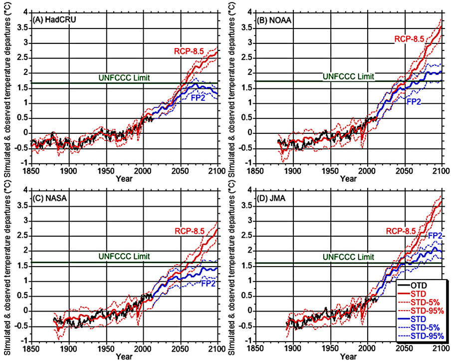
Figure 7. Observed departure (OTD, black line) and simulated departure (STD, red and blue lines) of global-mean nearsurface temperature from the 1961-1990 average. The simulated temperature departure is due to: 1) emissions of greenhouse gases, aerosol precursors, land-use changes, solar-cycle-caused solar-irradiance variations, and volcanoes from to through 2012 (Causes 2); 2) emissions of greenhouse gases and aerosol precursors for the Reference case of FP1/FP2 (red lines) and the Mitigation case of FP2 (blue lines) from 2013 to 2100; 3) solar-cycle-caused solar-irradiance variations from 2013 to 2100; 4) the sum of the sine-wave fits of QPO-1, QPO-2 and QPO-3 from to through 2100; and 5) the 90% confidence interval (STD-5% and STD-95%) for the unpredictable natural variability from to through 2100: (A) HadCRU [to = 1850, ΔT2x = 1.61˚C]; (B) NOAA [to = 1880, ΔT2x = 1.99˚C]; (C) NASA [to = 1880, ΔT2x = 1.45˚C] and (D) JMA [to = 1891, ΔT2x = 2.01˚C]. The sine-wave fit of QPO-1 for NOAA, NASA and JMA is the sine-wave fit for HadCRU shown in Figure 3. The 2˚C limit adopted by the UN Framework Convention on Climate Change is shown by the green line.
begin to deal with it.
For the Global Warming Problem, Phase 1—Ignorance —began with the onset of the Industrial Revolution circa 1750. In Phase 1 we were ignorant of the climatic consequences of our burning fossil fuel—coal, oil and natural gas. Phase 1 ended in 1979 with the publication of the first report on Global Warming by the National Research Council of the US Academy of Sciences, the so-called “Charney Report” named after Jule Charney, the chair of the ad hoc study group that wrote the report [22].
Phase 2—Uncertainty—began with the Charney Report in 1979. In Phase 2 we understood that burning fossil fuels would have climatic consequences, but we were uncertain about the scope and magnitude of those conesquences. Phase 2 is now ending, and Phase 3—Resolution—is beginning, because we can now bound the Global Warming Problem. Not only can we project the human contribution thereto—the source of the Problem— we can now project the natural variability and, thereby, bound the Problem into the future.
In so doing we can see that we cannot relegate the Global Warming Problem to the dustbin of problems that are too small to be of our concern. Rather, we can now see that absent any action by humanity to deal with the Global Warming Problem, it will exceed the maximum 2˚C global warming adopted by the United Nations Framework Convention on Climate Change “to prevent dangerous anthropogenic interference with the climate system”, and it will do so sometime between 2034 and 2076. Accordingly, it is time to begin to deal with the Global Warming Problem by adopting our Revised Fair Plan to Safeguard Earth’s Climate, FP2, which entails making the transition from the Fossil-fuel Age to the Post Fossil-fuel Age within this century, by phasing out the emission of greenhouse gases from 2020 to 2100.
6. Conclusions
In this paper we have used Singular Spectrum Analysis to analyze four observational datasets of global-mean near-surface temperature—the HadCRU, NOAA, NASA and JMA datasets. For each dataset we have found a trend and several quasi-periodic oscillations or QPOs. As we have shown previously in Causes 2 [3], the trend for each dataset is caused by human beings, predominantly by their emission of greenhouse gases (GHGs), but also by their emission of aerosol-precursor gases and land-use changes. The longest-period and largest-amplitude QPO is properly revealed by the HadCRU dataset which begins in 1850. QPO-1 is not properly revealed by the NOAA and NASA datasets, which begin in 1880, or by the JMA dataset which begins in 1891. Accordingly we recommend that the starting year of the NOAA, NASA and JMA datasets be extended back at least to 1850.
QPOs 1, 2 and 3 are sufficiently regular that each can be fit by a sine wave that can then be used to predict their future behavior year by year. The higher-order QPOs are not sufficiently regular to be predicted year by year into the future. But they and the remainder of the observed temperature departures can be predicted statistically on a non-year-by-year basis.
We project the human-caused changes in global-mean near-surface temperature across the 21st century for two scenarios of future emissions of greenhouse gases and aerosol-precursor gases, as well as for the 11-year solar sunspot cycle. One scenario is the Representative Concentration Path 8.5 scenario that we used as the Reference scenario in our FP1 and FP2 papers. The other scenario is the FP2 scenario that phases out the emission of greenhouse gases and aerosol-precursor gases from 2020 through 2100 in a fair manner such that the global-mean temperature change from preindustrial time does not exceed the 2˚C limit adopted by the UN Framework Convention on Climate Change “to prevent dangerous anthropogenic interference with the climate system” [9]. The FP2 scenario crafts the trade-adjusted cumulative emission of GHGs by the developing (so-called nonAnnex B or nAB) countries to be equal to trade-adjusted cumulative emission of GHGs by the developed (annex B or AB) countries. This is achieved by designing the emission-phaseout-intensity for the nAB countries from unity in 2020 to zero in 2100 using a cubic function of time, this in contrast to the linear-in-time emissionphaseout-intensity for the AB countries.
To the human-caused increases in global-mean, nearsurface temperature we add the non-human-caused changes therein by QPOs 1, 2 and 3. We convert this predictable part of the temperature change to temperature departure from the 1961-90 mean temperature as we have done heretofore [1,3,10]. We then subtract the observed temperature departures from the simulated temperature departures and fit the cumulative distribution function for the difference by a Normal distribution. The resulting fit is found to be excellent with a coefficient of determination larger than 0.99. To the predictable part of the projected change in temperature across the 21st century we add the unpredictable part in terms of its 5th and 95th percentiles.
We find that we are now entering the Third Phase of Learning—Resolution—wherein the signal of humancause global warming has, or soon will, swamp the noise of natural variability. Accordingly, it is now time for the UN Framework Convention on Climate Change to formulate an international agreement that phases out the emission of greenhouse gases from 2020 through 2100 following our Revised Fair Plan to Safeguard Earth’s Climate.
REFERENCES
- N. G. Andronova and M. E. Schlesinger, “Causes of Temperature Changes during the 19th and 20th Centuries,” Geophysical Research Letters, Vol. 27, No. 14, 2000, pp. 2137-2140. doi:10.1029/2000GL006109
- S. F. Singer, Ed., “Nature, Not Human Activity, Rules the Climate: Summary for Policymakers of the Report of the Nongovernmental International Panel on Climate Change,” Heartland Institute, Chicago, 2008, 50 p.
- M. J. Ring, D. Lindner, E. F. Cross and M. E. Schlesinger, “Causes of the Global Warming Observed Since the 19th Century,” Atmospheric and Climate Sciences, Vol. 2, No. 3, 2012, pp. 401-415. doi:10.4236/acs.2012.24035
- A. Revkin, “A Climate Scientist Proposes a ‘Fair Plan’ for Limiting Warming,” Dot Earth Blog, New York Times, 2012. http://dotearth.blogs.nytimes.com/2012/12/04/a-climate-scientist-proposes-a-fair-plan-for-limiting-warming/
- A. Revkin, “E-Mail Communication to Michael Schlesinger,” 2013.
- M. E. Schlesinger, M. J. Ring and E. F. Cross, “A Fair Plan for Safeguarding Earth’s Climate,” Journal of Environmental Protection, Vol. 3, No. 6, 2012, pp. 455-461. doi:10.4236/jep.2012.36055
- M. E. Schlesinger, M. J. Ring and E. F. Cross, “A Revised Fair Plan to Safeguard Earth’s Climate,” Journal of Environmental Protection, Vol. 3, No. 10, 2012, pp. 1330- 1335. doi:10.4236/jep.2012.310151
- United Nations, “United Nations Framework Convention on Climate Change,” 1992. http://unfccc.int/resource/docs/convkp/conveng.pdf.
- United Nations, “Report of the Conference of the Parties on Its Sixteenth Session. Addendum Part Two: Action Taken by the Conference of the Parties at Its Sixteenth session,” 2010. http://unfccc.int/meetings/cancun_nov_2010/meeting/6266/php/view/reports.php
- M. E. Schlesinger and N. Ramankutty, “An Oscillation in the Global Climate System of Period 65 - 70 Years,” Nature, Vol. 367, 1994, pp. 723-726. doi:10.1038/367723a0
- M. E. Schlesinger, N. G. Andronova, B. Entwistle, A. Ghanem, N. Ramankutty, W. Wang and F. Yang, “Modeling and Simulation of Climate and Climate Change,” In: G. Cini Castagnoli and A. Provenzale, Eds., Past and Present Variability of the Solar-Terrestrial System: Measurement, Data Analysis and Theoretical Models, Proceedings of the International School of Physics Enrico Fermi CXXXIII, IOS Press, Amsterdam, 1997, pp. 389- 429.
- C. P. Morice, J. J. Kennedy, N. A. Rayner and P. D. Jones, “Quantifying Uncertainties in Global and Regional Temperature Change Using an Ensemble of Observational Estimates: The HadCRUT4 Dataset,” Journal of Geophysical Research, Vol. 117, No. D8, 2012. doi:10.1029/2011JD017187
- T. M. Smith, R. W. Reynolds, T. C. Peterson and J. H. Lawrimore, “Improvements to NOAA’s Historical Merged Land-Ocean Surface Temperature Analysis,” Journal of Climate, Vol. 21, No. 10, 2008, pp. 2283-2296. doi:10.1175/2007JCLI2100.1
- J. Hansen, R. Ruedy, M. Sato and K. Lo, “Global Surface Temperature Change,” Reviews of Geophysics, Vol. 48, No. 4, 2010, Article ID: RG4004. doi:10.1029/2010RG000345
- K. Ishihara, “Calculation of Global Surface Temperature Anomalies with COBE-SST,” (Japanese) Weather Service Bulletin, Vol. 73, 2006, pp. S19-S25.
- K. Ishihara, “Estimation of Standard Errors in Global Average Surface Temperature,” (Japanese) Weather Service Bulletin, Vol. 74, 2007, pp. 19-26.
- M. Ghil and R. Vautard, “Interdecadal Oscillations and the Warming Trend in the Global Temperature Time Series,” Nature, Vol. 350, 1991, pp. 324-327. doi:10.1038/350324a0
- A. Korobeynikov, “Computationand Space-Efficient Implementation of SSA,” Statistics and Its Interface, Vol. 3, No. 3, 2010, pp. 357-368.
- A. Korobeynikov, “A Collection of Methods for Singular Spectrum Analysis, in Package ‘Rssa’,” 2013, pp. 1-34. http://cran.r-project.org/web/packages/Rssa/Rssa.pdf
- R. D. C. Team, “R: A Language and Environment for Statistical Computing,” R Foundation for Statistical Computing, Vienna, 2011.
- “Kaleidagraph,” Synergy Software.
- National Research Council, “Carbon Dioxide and Climate: A Scientific Assessment,” US National Academy of Sciences, Washington DC, 1979, 22 p.
- M. Ghil, R. Allen, M. D. Dettinger, K. Ide, D. Kondrashov, M. E. Mann, A. W. Robertson, A. Saunders, Y. Tian, F. Varadi and P. Yiou, “Advanced Spectral Methods for Climatic Time Series,” Reviews of Geophysics, Vol. 40, No. 1, 2002, pp. 3-1-3-41. doi:10.1029/2000RG000092
- C. L. Keppenne and M. Ghil, “Adaptive Spectral Analysis and Prediction of the Southern Oscillation Index,” Journal of Geophysical Research, Vol. 367, No. D18, 1992, pp. 20449-20554. doi:10.1029/92JD02219
- M. Ghil, “The SSA-MTM Toolkit: Applications to Analysis and Prediction of Time Series,” Proceedings of the SPIE—The International Society for Optical Engineering, Applications of Soft Computing, Vol. 3165, 1997, pp. 216-230.
Appendix: Representation of the QPOs
We have examined seven methods of representing QPOs using three different approaches.
The first approach is an SSA-forecasting approach implemented in the RSSA package [18,19] of the statistical software R [20] and yields “the new series which is expected to ‘continue’ the current series” [19] based on a given decomposition. Two distinct algorithms are evaluated, “SSA-vector” and “SSA-recurrent”. SSA-vector “sequentially projects the incomplete embedding vectors (either from the original or reconstructed series) onto the subspace spanned by the selected eigen-triples of the decomposition to derive the missed (ending) values of the such vectors” [19]. SSA-recurrent “continues the set of vectors in the subspace spanning the chosen eigenvectors (…) and then derive the series out of this extended set of vectors” [19].
The second approach is built on the idea that the QPOs are narrowband time series and therefore can be predicted fairly well by fitting a low-order auto-regressive (AR) process to the QPOs [23]. The method has been successfully used by [24] to forecast the SOI time series with considerable skill for 30 to 36 months. However [25] concluded that the instrumental temperature record is not long enough to determine its quasi-periodic components reliably enough to allow for a skillful decadal or longer forecast.
Because our temperature record is more than 20 years longer than that of [25], QPOs 1, 2 and 3 are extracted, fitted with an AR process, and the coefficients thereof are used to predict their future evolution. This approach is implemented in the statistical software R [20], and the “AR-Burg”, “AR-OLS”, “AR-MLE” and “AR-YuleWalker” methods of fitting the AR-model are evaluated.
The order M of the AR process is either automatically determined using the Akaike Information Criterion or fixed.
Finally, since QPO-1, QPO-2 and QPO-3 are quite periodic, each is fitted with a sine function that is used to extrapolate into the future.
The forecast skill for the above methods is assessed for 5, 10 and 20-year periods using the HadCRUT4 record. This record is truncated to: 1) 1850 to 1990; 2) 1850 to 2000 and 3) 1850 to 2005 and SSA is used to determine the corresponding “truncated” QPOs 1 through 3. These truncated QPOs are then forecast into the future and are compared to the QPOs of the 1850-2010 time series. The forecasting skills of the different methodologies are evaluated using: 1) visual inspection, V; 2) root-meansquare errors, R; and 3) the correlation coefficient, ρ. In Table A1 we summarize our skill assessment based on four criteria: “+”, “0”, “−” and “/”. A “+” indicates good V, small R and ρ > 0.8. A “0” means a neutral V, that is, neither good nor bad; an average R compared to the overall distribution of R for this particular skill test, and 0.3 < ρ < 0.8. A “−” signifies poor V, large R and ρ < 0.3. A “/” indicates the failure to fit the corresponding QPO. The Score equals the sum of +’s (each = 1), 0’s (each = 0), −’s (each = −1) &/’s (each = −2).
The best method by far is “Sine”, followed by “SSARecurrent”, “AR-Burg” and “AR-YW”. However, the latter is very dissipative in time and hence not applicable for more than a decade. The “SSA-Recurrent” approach shows considerable skill in forecasting QPO-1 for 5 and 10 years, but tends to underestimate the actual amplitudes of QPO-2 and QPO-3. The latter is also a problem of the “SSA-Vector” approach. The other two methods fail the majority of skill tests; “AR-MLE” is especially unsuccessful in fitting an AR process to QPO-1.
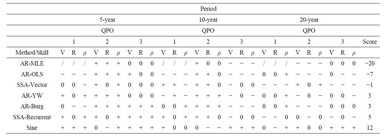
Table A1. Skill assessment for 5-year, 10-year and 20-year projections based on: 1) visual inspection, V; 2) root-mean-square error, R; and 3) correlation coefficient, ρ. A “+” indicates good V, small R and ρ > 0.8. A “0” means a neutral V, with an average R and 0.3 < ρ < 0.8. A “−” signifies poor V, large R and ρ < 0.3. A “/” indicates the failure to fit the corresponding QPO. The Score equals the sum of +’s (each = 1), 0’s (each = 0), −’s (each = −1) &/’s (each = −2).