Journal of Signal and Information Processing
Vol.4 No.2(2013), Article ID:31295,6 pages DOI:10.4236/jsip.2013.42028
Adaptive Matrix/Vector Gradient Algorithm for Design of IIR Filters and ARMA Models*
![]()
1VTT Technical Research Centre of Finland, Espoo, Finland; 2Department of Applied Physics, University of Eastern Finland, Kuopio, Finland.
Email: juuso.olkkonen@vtt.fi, hannu.olkkonen@uef.fi
Copyright © 2013 Juuso T. Olkkonen et al. This is an open access article distributed under the Creative Commons Attribution License, which permits unrestricted use, distribution, and reproduction in any medium, provided the original work is properly cited.
Received January 26th, 2013; revised February 28th, 2013; accepted March 10th, 2013
Keywords: Adaptive Signal Processing; Gradient Algorithm; SVD; Noise Rejection
ABSTRACT
This work describes a novel adaptive matrix/vector gradient (AMVG) algorithm for design of IIR filters and ARMA signal models. The AMVG algorithm can track to IIR filters and ARMA systems having poles also outside the unit circle. The time reversed filtering procedure was used to treat the unstable conditions. The SVD-based null space solution was used for the initialization of the AMVG algorithm. We demonstrate the feasibility of the method by designing a digital phase shifter, which adapts to complex frequency carriers in the presence of noise. We implement the half-sample delay filter and describe the envelope detector based on the Hilbert transform filter.
1. Introduction
Theory and design of the adaptive FIR (finite impulse response) filters is recently impacted by high speed digital communication systems such as video and image processing. The multi-rate data acquisition VLSI devices based on the tree structured discrete wavelet transforms (DWTs) have significantly advanced with the adaptive techniques such as data compression, adaptive noise cancellation and channel equalization [1-3].
The IIR (infinite impulse response) filter structures are not as popular as the FIR filters in signal decomposition and multi-scale analysis. Also the adaptive IIR filters are generally only marginally stable since the poles may travel outside the unit circle during the adaptation process. However, recently the time reversed filtering procedure was introduced, which enables the implementation of the IIR filters having poles outside the unit circle [4]. The IIR filter structures have many advantages over the FIR filters. Usually the equal performance (e.g. convergence rate and adaptation error can be obtained by a considerably lower number of filter coefficients compared with the FIR filters.
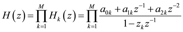
The IIR filter consists of the transfer function
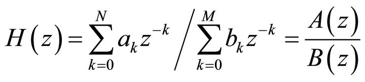 (1)
(1)
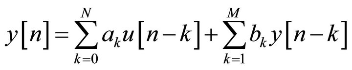
The output of the filter in discrete-time domain can be computed recursively as
 . (2)
. (2)
In this equation  and
and  are the coefficients of the nominator and denominator polynomials,
  and
and  are the input and output signals. In process, control literature (2) is usually named as autoregressive moving average (ARMA) signal model.
In this work, we introduce an adaptive matrix/vector gradient (AMVG) algorithm for design of IIR filters and ARMA systems. We apply the SVD-based null space solution for the initialization of the AMVG algorithm. Finally, we prove the usefulness of the AMVG algorithm in the design of digital phase shifter,
2. IIR Filter (ARMA Model) Formulation
The input-output relation of the discrete-time IIR filter (1) can be written as
 (3)
(3)
where  and
and  denote z-transforms of the input and output signals. This yields
 (4)
(4)
By defining the Hankel data matrices
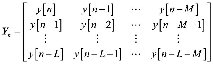 (5)
(5)
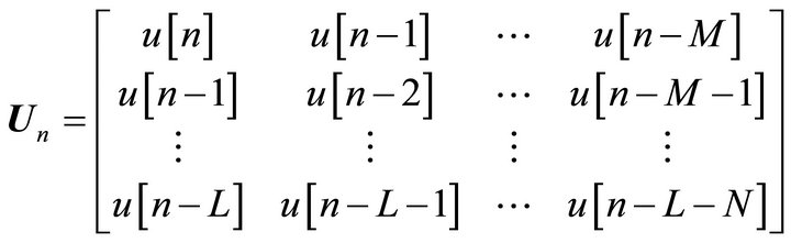 (6)
(6)
where  and the coefficient vectors
 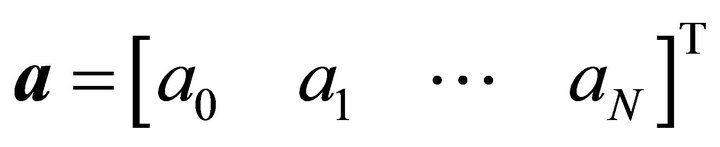 and
and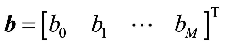 , we obtain
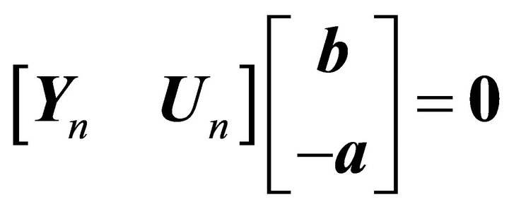 (7)
(7)
where  is a zero vector.
3. SVD-Based Initialization Method
In the following we describe the SVD-based null space solution of the coefficient vectors in (7). Let us replace the input-output data matrix by a short notation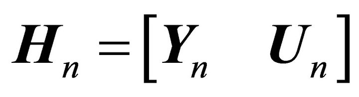 . By applying the singular value decomposition (SVD) we have
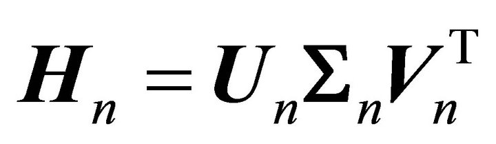 , where matrices
 and
and  contain the left and right singular vectors (column vectors) and matrix
  the singular values in descending order. Matrices
  and
and  are unitary:
  and
and , where
  denotes the unity matrix. This gives
 , i.e.
  . Finally we may write
 (8)
(8)
for . Equation (8) forms the basis for the SVD-based initialization method. By searching very small singular value
 , the right singular vector
  equals vector
  in (7) yielding the solution for the coefficient vectors. In the presence of noise the dimensions of the data matrix
  should be selected so that there appears only one tiny singular value. This can be also achieved by zeroing the rest of the tiny singular values in SVD decomposition of the data matrix.
In applications where the coefficient vector is time varying, the SVD computation is unacceptably time consuming. Therefore the SVD-based solution is only justified in the initialization of the IIR filter design. In the following we describe a fast matrix/vector gradient (AMVG) algorithm for adaptive computation of the IIR filter parameters.
4. Adaptive Matrix/Vector Gradient Algorithm
For adaptation of the ![]() and
and  coefficient vectors we define the adaptation error vector
  as
as
 (9)
(9)
The mean square error (MSE) is computed as . The coefficient vectors are then updated by the gradient algorithm as
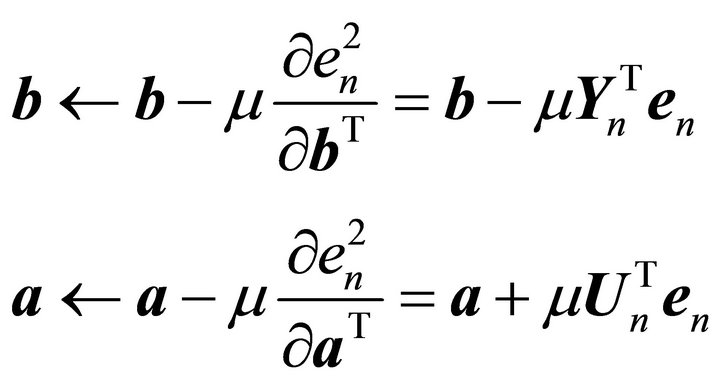 (10)
(10)
where  denotes the adaptation gain factor. This is followed by the gain normalization
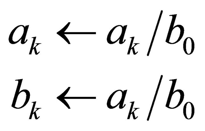 (11)
(11)
The normalization (11) fixes the coefficient . In our experience the post normalization of the gain warrants more reliable convergence of the algorithm compared with fixing directly
  in (10). Since the gradient algorithm is based on the use of the same data matrices
  and
and  as in the SVD-based solution, the initial selection of the coefficient vectors in (10) may be the same as in the SVD-based solution. Using arbitrary coefficient vectors as initial guess would possibly result in the convergence to the local minimum.
5. Implementation of the IIR Filters and ARMA Models
Many IIR filters designed by the present method are not readily implementable, since the poles may lie outside the unit circle. In this case the poles outside the unit circle must be considered separately. The denominator polynomial is divided into anticausal (AC) and causal (C) parts
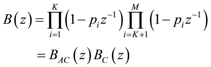 (12)
(12)
where the roots 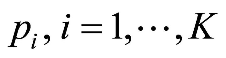 are outside the unit circle. The anticausal filter
  can be implemented by the time reversed filtering procedure [4]. The anticausal filter
  in (12) as a cascade realization
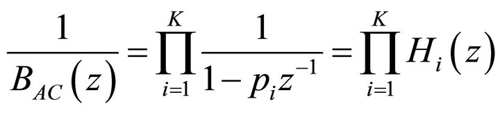 (13)
(13)
where the poles  are outside the unit circle. The
  filters in (13) can be implemented by the following time reversed filtering procedure. First we replace z by
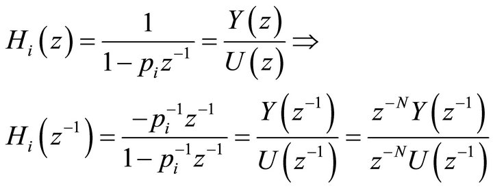 (14)
(14)
where  and
and  are z-transforms of the input
  and output
  signals
 .
.
 and
and  are the z-transforms of the time reversed input
  and time reversed output
 . The
. The  filter is stable having a pole
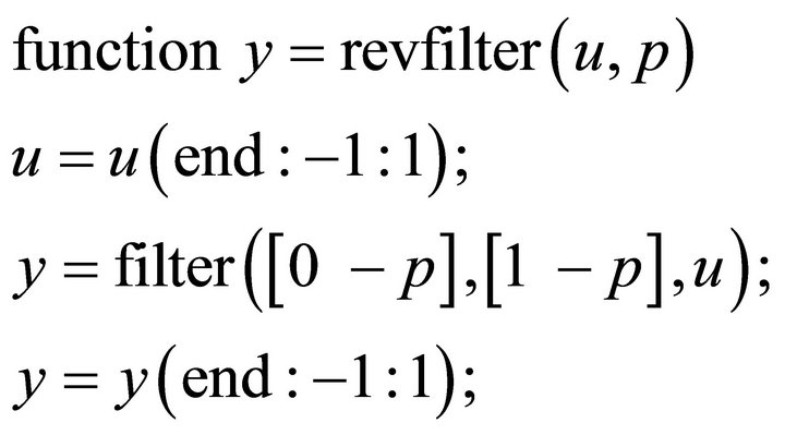
  inside the unit circle. The following Matlab program revfilter.m demonstrates the computation procedure:
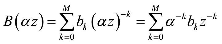
In many IIR filter realizations the poles of the transfer function lie close to the unit circle and unstable conditions and oscillations may occur when filtering timevarying signals with abrupt changes and discontinuities. Let us consider the modification of the denominator polynomial of the IIR filter where the z-transform variable is multiplied by 
 (15)
(15)
The roots of the modified polynomial are transferred towards the origin of the unit circle, which increases the inherent stability of the filter. We may observe that this is equivalent if we weight the IIR filter coefficients as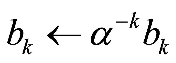 , which can be directly inserted to the gain normalization procedure (11).
The computation speed of the AMVG algorithm can be increased by using the sequential blocks of input and output data. We may define the data matrices as  and
and , where
  and W is the length of the data block.
With a slight modification the AMVG algorithm can be implemented to state-space system identification. Let us define the state-space model as
 (16)
(16)
where the state vector , the state transition matrix
 , matrices
 . Vectors
  contain the input
  and output
  signals. Vector
  is a random zero mean observation noise sequence. By defining the Hankel data matrices (5) and (6) the ARMA model polynomials (1) can be identified. Then we may formulate (16). However, it should be pointed out that the state-space solution is not unique. We prefer the companion matrix structure of the state transition matrix
 , which allows the direct insertion of the polynomial coefficients in (1). Fast computational algorithms are presented in [5,6].
6. Design Example: A Digital Phase Shifter
Our purpose is to design a digital phase shifter, which adapts to M frequency carriers buried in heavy noise. The prototype IIR filter has the transfer function
 (17)
(17)
The output signal  has the
  phase shift in respect to the input signal
 . Hence, the envelope
  of the carrier wave is obtained as
 (18)
(18)
The tracking performance of the adaptive matrix/vector gradient algorithm is illustrated in Figure 1 for . Blue waveform denotes the input signal and red the output of the digital filter (17). The input signal in the upper view contains only a low level noise component, whereas in the lower view the input signal is buried by
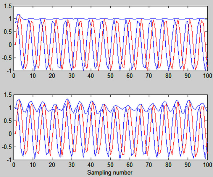
Figure 1. The performance of the AMVG algorithm in the design of the digital phase shifter.
heavy noise. The envelope in upper picture attains a constant level in about 7 - 10 rounds. In lower picture the envelope is clearly fluctuating in the presence of high noise component.
7. Design Example: A Half-Sample Delay Filter
Our purpose is to optimize the digital IIR filter coefficients for half-sample operation. For the input signal , the filter output should equal
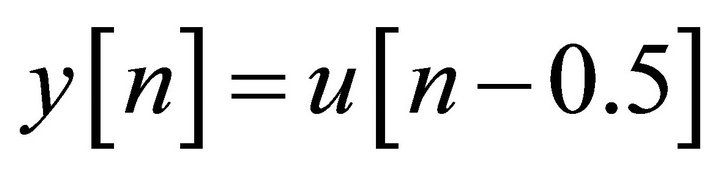 . The prototype was selected as
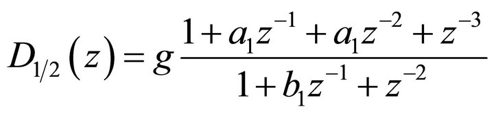 (19)
(19)
where g is the gain factor. Due to the symmetric structure the prototype contains only three adjustable parameters. The test signal was a neuroelectric waveform recorded from the frontal cortex at sampling rate of 400 Hz with a 14 bit ADC. The experimental arrangement is described in detail in [18]. The input signal comprised of the even samples of the EEG and the output from the odd samples, correspondingly. After 10 - 14 rounds the parameter values converged to (mean![]() 1 s.d.)
1 s.d.)  and
and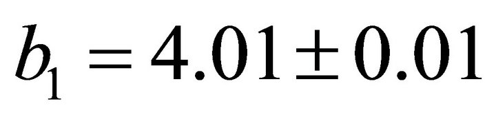 .
.
The results correlated highly significantly (intraclass correlation coefficient ) with the data obtained by the B-spline polyphase decomposition method [7].
8. Design Example: Envelope Detector
The validity of the adaptive half-sample delay filter (18) was tested by the signal  where
where ![]() varied randomly in the range 0.9 - 1.1. The interpolation error was between
varied randomly in the range 0.9 - 1.1. The interpolation error was between  - 1.2 percent. In our recent work [8] we discovered a novel way to construct Hilbert transform filter as
 (20)
(20)
Figure 2 shows a typical test waveform and the envelope based on the adaptive Hilbert transform filter (19).
9. Discussion
In signal processing society the state-of-the art IIR filter and ARMA model design methods have a rich literature. Among adaptive filters the Kalman filter has a predominant role [9-13]. In many industrial and medical systems the least mean square (LMS) and recursive least squares (RLS) algorithms have their earned position [14,15]. A common disadvantage to all adaptive IIR structures is the relatively slow recovery from the anomalies occurring in the measurement signal such as transients, edges and
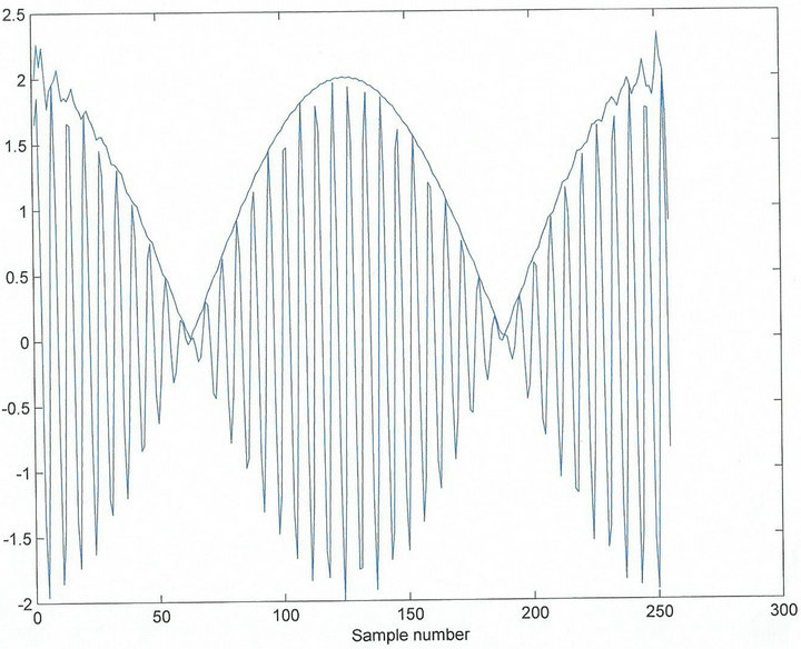
Figure 2. The envelope of the sinusoidal signal with randomly varying frequency.
other discontinuities.
In this work we introduced the SVD-based null space method for initialization of the model parameters. As a clear advantage is the SVD-based method is the estimation of the model order. The number of non-zero singular values matches the rank of the data matrix, which equals the model order. The SVD-based initialization method rapidly recovers the IIR (ARMA) signal model after a mismatch. It should be pointed out that in the presence of extreme heavy noise, the SVD-based initialization usually achieves the correct filter coefficients for the data matrix , which contains only one tiny singular value and the rest of the data matrix can be considered to belong to the signal subspace. In the uptake process (10) the data matrices
  and
and  are not noise free and the AMVG algorithm does not necessarily converge or has a poor convergence rate.
Compared with the previous gradient based adaptive algorithms such as LMS and RLS, the main difference in AMVG algorithm is involved in the definition of the system transfer function (1). In LMS algorithm the nominator contains only the gain factor (autoregressive signal model), but in AMVG algorithm the nominator is defined as polynomial . The measurement signals may contain a relatively large noise component and adaptation error in LMS algorithm is directly affected by noise. In definition (7) both the input and output signals are subspace reduced [16-18] by the SVD-based initialization method and the noise is not directly imposed in the adaptation error.
In this work we demonstrated the feasibility of the AMVG algorithm in the design of the digital phase shifter. An evident application would be the noise cancellation equipment, where the measured environmental noise serves as an input signal . The phase shifted output signal
  drives the loudspeaker and due to the negative feedback, the equipment eliminates noise in the measurement site. In previous noise reduction systems the fractional delay filters [4,19,20] have been implemented for that purpose.
The second example considered the construction of the half-sample filter, where three parameters in the AMVG algorithm were successfully optimized for a neuroelectric waveform [7]. The half-sample delay filter has in an important role in the computation of the shift invariant multi-scale wavelets. We have applied the discrete B-spline polyphase decomposition for that purpose [7]. Our preliminary tests reveal that the AMVG algorithm competes extreme well with the B-spline half-sample delay filters. The neuroelectric discharge contains fast repetitive transients with exponentially decaying activity [7,21]. The AMVG algorithm converges to the asymmetric shape of neuronal spikes. The symmetric B-spline quadrature mirror filters (QMFs) with integer coefficients cannot perform so well. However, in practice the difference is small and the EEG analysis based on the AMVG algorithm does not overdrive the instrumention based on the B-spline signal processing [22].
Finally, we implemented the adaptive half-sample delay filter (18) for computation of the envelope of the sinusoid with varying frequency. The frequency jittering signals are common in industrial and medical instrumentation. For example the 50 Hz pick-up will interfere the ambulatory measurement of the ECG, EEG and EMG waveforms [1-3,21]. An efficient noise rejection method is yielded by adapting the signal to the transfer function  in (17). A noise free signal is obtained by filtering the original waveform by the pole cancellation filter
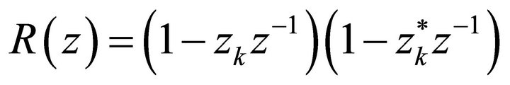 , where
  denotes complex conjugation. The pole
  in (17) corresponds the complex waveform
 , where
 . The frequency
  [Hz] should be close to 50 Hz.
As an important application of the AMVG algorithm is the prediction of the signal waveform for example in process control. For the input signal  the system adapts to the output
 , where
  is the prediction step.
After convergence of the AMVG algorithm, we may use the result to predict the future behaviour of the process. Usually this gives prophylactic information for the system service planning etc. As an extra value, the magniture and phase response of the system can be computed applying e.g. Matlab freqz  instruction.
REFERENCES
- J. T. Olkkonen, “Discrete Wavelet Transforms: Theory and Applications,” Intech, 2011.
- H. Olkkonen, “Discrete Wavelet Transforms: Algorithms and Applications,” Intech, 2011, 296 p.
- H. Olkkonen, “Discrete Wavelet Transforms: Biomedical Applications,” Intech, 2011, 366 p.
- J. T. Olkkonen and H. Olkkonen, “Fractional Delay Filter Based on the B-Spline Transform,” IEEE Signal Processing Letters, Vol. 14, No. 2, 2007, pp. 97-100. doi:10.1109/LSP.2006.882103
- H. Olkkonen, S. Ahtiainen, J. T. Olkkonen and P. Pesola, “State-Space Modelling of Dynamic Systems Using Hankel Matrix Representation,” International Journal of Computer Science & Emerging Technologies, Vol. 1, No. 4, 2010, pp. 112-115.
- J. T. Olkkonen and H. Olkkonen, “Least Squares Matrix Algorithm for State-Space Modelling of Dynamic Systems,” Journal of Signal and Information Processing, Vol. 2, No. 4, 2011, pp. 287-291. doi:10.4236/jsip.2011.24041
- H. Olkkonen and J. T. Olkkonen, “Shift-Invariant B-Spline Wavelet Transform for Multi-Scale Analysis of Neuroelectric Signals,” IET Signal Processing, Vol. 4, No. 6, 2010, pp. 603-609. doi:10.1049/iet-spr.2009.0109
- J. T. Olkkonen and H. Olkkonen, “Complex Hilbert Transform Filter,” Journal of Signal and Information Processing, Vol. 2, No. 2, 2011, pp. 112-116.
- F. Daum, “Nonlinear Filters: Beyond the Kalman Filter,” IEEE A&E Systems Magazine, Vol. 20, No. 8, 2005, pp. 57-69.
- A. Moghaddamjoo and R. Lynn Kirlin, “Robust Adaptive Kalman Filtering with Unknown Inputs,” IEEE Transactions on Acoustics, Speech and Signal Processing, Vol. 37, No. 8, 1989, pp. 1166-1175. doi:10.1109/29.31265
- J. L. Maryak, J. C. Spall and B. D. Heydon, “Use of the Kalman Filter for Interference in State-Space Models with Unknown Noise Distributions,” IEEE Transactions on Automatic Control, Vol. 49, No. 1, 2005, pp. 87-90.
- R. Diversi, R. Guidorzi and U. Soverini, “Kalman Filtering in Extended Noise Environments,” IEEE Transactions on Automatic Control, Vol. 50, No. 9, 2005, pp. 1396- 1402. doi:10.1109/TAC.2005.854627
- D.-J. Jwo and S.-H. Wang, “Adaptive Fuzzy Strong Tracking Extended Kalman Filtering for GPS Navigation,” IEEE Sensors Journal, Vol. 7, No. 5, 2007, pp. 778-789. doi:10.1109/JSEN.2007.894148
- S. Attallah, “The Wavelet Transform-Domain LMS Adaptive Filter with Partial Subband-Coefficient Updating,” IEEE Transactions on Circuits and Systems II, Vol. 53, No. 1, 2006, pp. 8-12. doi:10.1109/TCSII.2005.855042
- H. Olkkonen, P. Pesola, A. Valjakka and L. Tuomisto, “Gain Optimized Cosine Transform Domain LMS Algorithm for Adaptive Filtering of EEG,” Computers in Biology and Medicine, Vol. 29, No. 2, 1999, pp. 129-136. doi:10.1016/S0010-4825(98)00046-8
- E. Biglieri and K. Yao, “Some Properties of Singular Value Decomposition and Their Applications to Digital Signal Processing,” Signal Processing, Vol. 18, No. 3, 1989, pp. 277-289. doi:10.1016/0165-1684(89)90039-X
- S. Park, T. K. Sarkar and Y. Hua, “A Singular Value Decomposition-Based Method for Solving a Deterministic Adaptive Problem,” Digital Signal Processing, Vol. 9, No. 1, 1999, pp. 57-63. doi:10.1006/dspr.1998.0331
- T. J. Willink, “Efficient Adaptive SVD Algorithm for MIMO Applications,” IEEE Transactions on Signal Processing, Vol. 56, No. 2, 2008, pp. 615-622. doi:10.1109/TSP.2007.907806
- T. J. Lim and M. D. Macleaod, “On Line Interpolation Using Spline Functions,” IEEE Signal Processing Society, Vol. 3, No. 5, 1996, pp. 144-146. doi:10.1109/97.491656
- J. T. Olkkonen and H. Olkkonen, “Fractional Time-Shift BSpline Filter,” IEEE Signal Processing Letters, Vol. 14, No. 10, 2007, pp. 688-691. doi:10.1109/LSP.2007.896402
- J. T. Olkkonen and H. Olkkonen, “Shift Invariant Biorthogonal Discrete Wavelet Transform for EEG Signal Analysis, Book Chapter 9,” In: J. T. Olkkonen, Ed., Discrete Wavelet Transforms: Theory and Applications, Intech, 2011. doi:10.5772/23828
- J. T. Olkkonen and H. Olkkonen, “Discrete Wavelet Transform Algorithms for Multi-Scale Analysis of Biomedical Signals, Book Chapter 4,” In: H. Olkkonen, Ed., Discrete Wavelet Transforms: Biomedical Applications, Intech, 2011.
NOTES
*This work was supported by the National Technology Agency of Finland (TEKES).