International Journal of Geosciences
Vol.4 No.2(2013), Article ID:29426,7 pages DOI:10.4236/ijg.2013.42042
Identification of Forerunners and Transmission of Energy to Tsunami Waves Generated by Instanteneous Ground Motion on a Non-Uniformly Sloping Beach
Department of Mathematics, Khalisani College, Chandannagar, India
Email: b.arghya@gmail.com
Received November 8, 2012; revised December 9, 2012; accepted January 11, 2013
Keywords: Tsunami Waves; Shallow Water Equations; Hankel Transform; Hankel Functions; Asymptotic Expansion
ABSTRACT
The problem of generation and propagation of tsunami waves is mainly focused on plane beach, there are very few analytical works where wave generation is considered on non-uniformly sloping beach and as a result those works might have failed to capture important facts which are influenced by bottom-slope of the beach. Some researchers provided solution to the forced long linear waves but on a beach with uniform slope while the importance of including variable bottom topography is mentioned by few researchers but they also stayed away from considering continuous variability of the ocean bed as they were studying runup problem. This paper analyzes tsunami waves which are generated by instantaneous bottom dislocation on a ocean floor with variable slope of the form , q > 0, r > 0. Attempts are made to find analytical solution of the problem and along the way tsunami forerunners are identified while investigating the short time wave behavior, not found even with constant slope beaches. In our study a rather significant phenomenon with regard to energy transmission to the waves at steady-state are observed with some notable features.
1. Introduction
The evaluation of the terminal effect of natural hazards remains one of the holy grails of geophysical research [1]. Needless to say tsunami is one such geophysical problem where uncertainties are yet to settle on the core areas of tsunami generation and propagation. Over the years mathematical complicacies have prevented researchers to do analytical work both in linear or non-linear version of the problem. As a consequence analytical works are far and few compared to the numerical studies of this genre of problems with more or less identical physical setting. Talking about previous work, at this stage, we wish to mention the seminal work of Tuck and Hwang [2] and also of Liu et al. [3] both provided analytical solution to the forced wave problem in a linear setting with uniform sloping beach. On the other hand Kanoglu and Synolakis [4] considered a piecewise continuous bathymetry to study long wave runup problem. Our interest is to study the generation and propagation of long waves due to underground sea bed dislocation on a variable ocean slope. The aim is to find an analytical solution and for that purpose we have restricted ourselves solving the linear shallow water equations with appropriate initial and boundary conditions. Here it would be quite interesting to point out that certain important parameters like tsunami wave runup can realistically be estimated staying well within the linear theory [5]. In this article we investigate generation of waves which are assumed to be caused by an instantaneous ground upheaval, along with a prescribed initial elevation and a velocity of the free surface at the instant before the ground begins to move. The problem is analyzed taking into account linear shallow water equation for a beach of variable slope , q > 0, r > 0, referred to horizontal and vertical directions as x-and y-axis respectively. In conformity with Tuck and Hwang’s analysis of long wave generation due to arbitrary ground motion over a uniformly sloping beach (r = 1), we first show that it is possible to find a non-singular solution of the problem for all time t when the ocean slope varies. Then by taking a very general type of time–dependent bottom dislocation we have been able to split the integrals in two parts one representing the waves due to free vibration which we claim to be the forerunners and the other as the forced wave part. These forerunners will dominate the wave-spectrum for first few minutes before the giant waves come and then will be dominated by the forced wave part, which is the other part of the wave. These forced waves ultimately catching up the free waves will occupy the whole spectrum beyond the half period of the quake forcing. An illustration of this has been shown by employing a particular type of bottom dislocation. Assuming a time periodic ground motion, we next show that a steady-state exists. At this stage we are confronted with a paradoxical result. Our solution at the steady-state shows a noteworthy feature of no transmission of energy from a finitely distributed time-periodic ground motion for a certain set of values of the disturbance function. This kind of paradox was first observed by Stoker for steady-state surface waves in infinitely deep water [6] and this peculiar ’resonance’ may perhaps be eliminated by assuming small viscosity of the fluid or by taking alongshore variations into account. Our attempt to find analytical solution of the problem helps us to understand the influence of variable bottom slope on wave elevation and velocity. Both the small-time and steady-state analysis of the problem performed here might be of some significance for the evolution of tsunami waves induced by near-shore earthquakes [7]. It will not be out of context to mention that although physical settings are different, the generation of long waves by variable atmospheric pressure distribution is analogous to the problem of tsunami formation by bottom displacement [8,9] and hence our solution may also prove pertinent to that direction. We have seen the devastation of the great Indian Ocean Tsunamis of 2004 and that of the more recent Japan earthquake, and has also observed the failure of the early warning system in quite a number of cases, keeping that in mind we hope these solutions can be used as a benchmark to all such numerical studies relating tsunami warning process. In passing, we wish to mention that in reality sea bottom profile is complex and is far from the general parabolic shape assumed here but this work can be considered as a first step, particularly in analytical sphere, towards including those complex curvilinear ocean floor associated with the bathymetric obstacles like island chain, rises and seamounts [10].
2. Problem and Its Solution
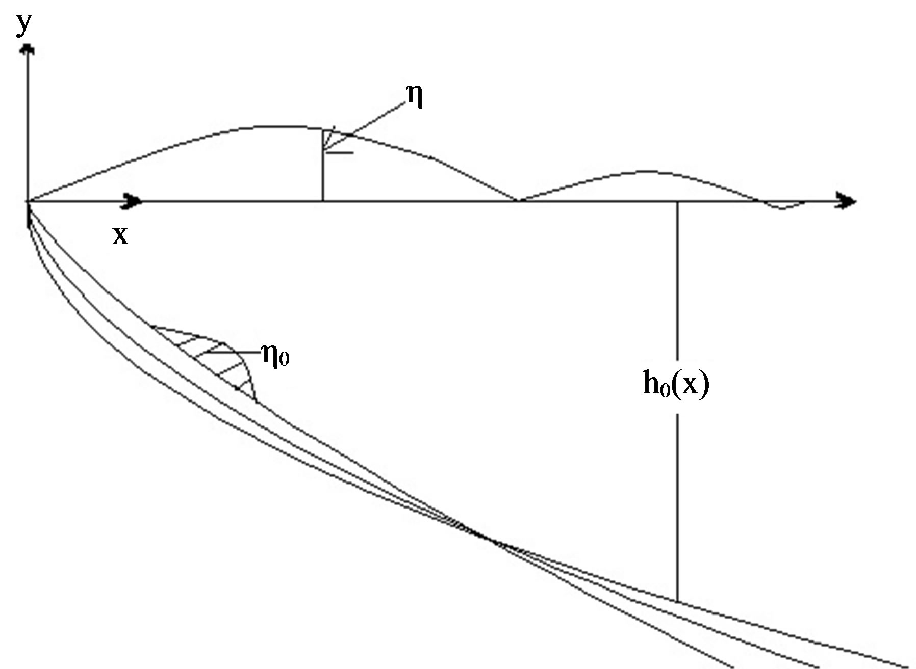
We take the vertical upward direction as the y-axis, and the undisturbed horizontal surface of the sea as the xz -plane of which the axis Oz is along the shoreline. The sea is supposed to be bounded by a beach of variable slope given by the equation y = h0 (x) at equilibrium (Figure 1).
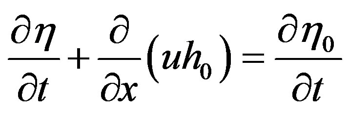
We assume a two-dimensional motion in which long waves are exited by a sudden bottom upheaval of height h0 (x, t) accompanied by an initial surface displacement h1(x) together with an initial vertical surface velocity h2 (x). If u(x, t) is the horizontal velocity, h(x, t) is the surface displacement and
 (1)
(1)
 (a)
(a)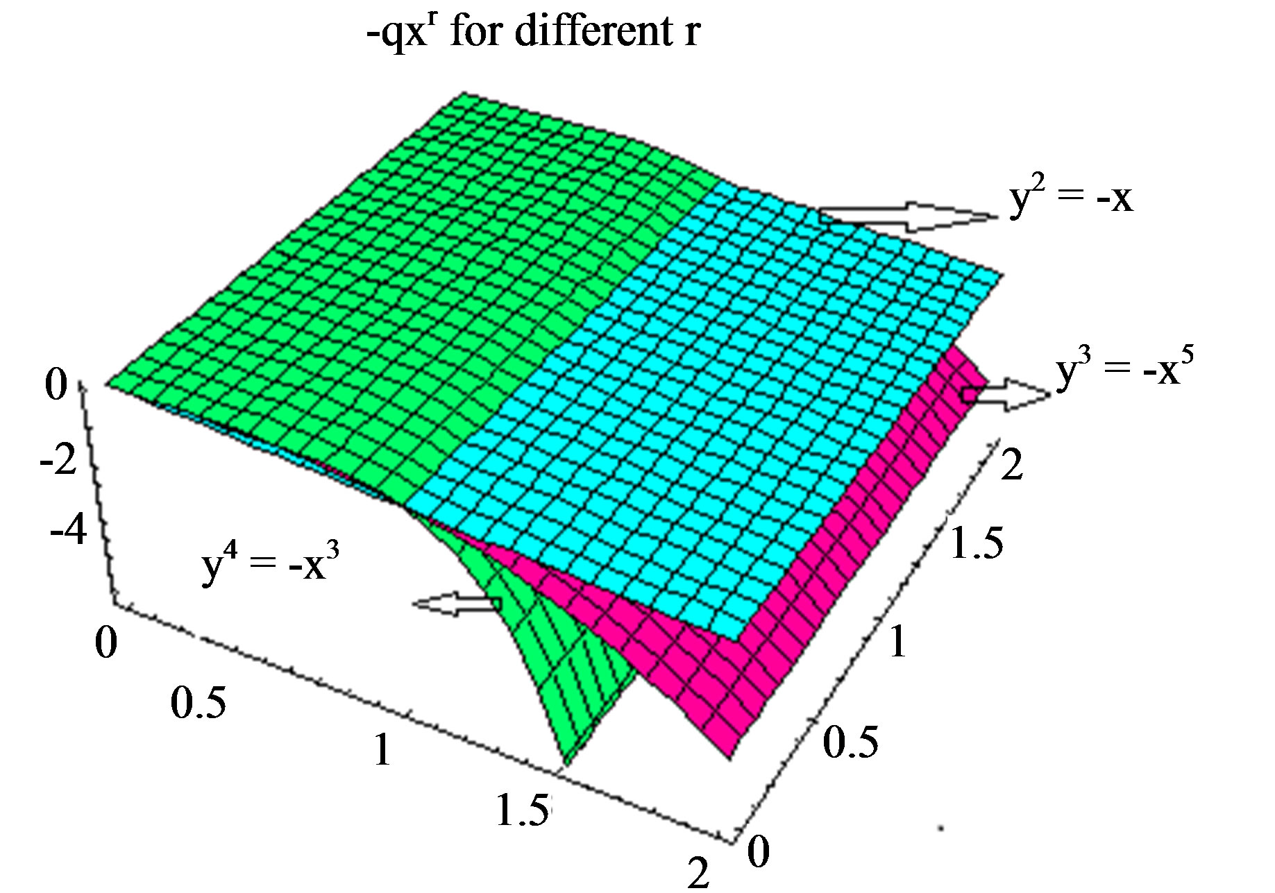 (b)
(b)
Figure 1. (a) The illustrative figure of the beach profile and the choice of axes; (b) This is a three-dimensional view of the bathymetry profile y = -qxr for different values of r.
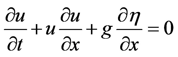
is the depth at the point x, at time t > 0, the non-linear shallow water equations are
 (2)
(2)
 . (3)
. (3)
At t = 0-, we have
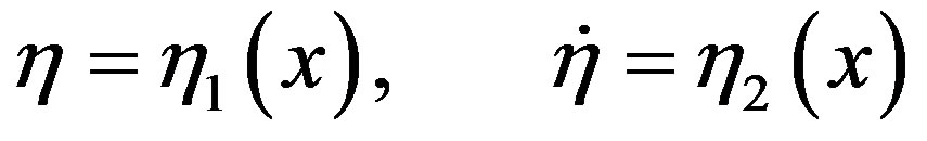 (4)
(4)
If  and
and  are small compared to
  and
and ![]() is small compared with the local wave speed
is small compared with the local wave speed , Equations (2) and (3), after using (1), may be linearised to
 , (5)
, (5)
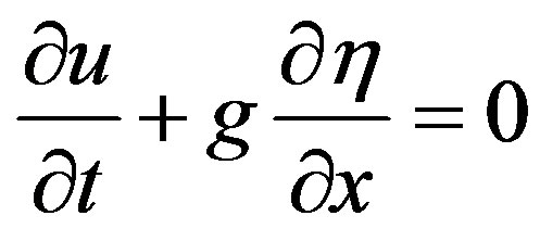 . (6)
. (6)
Eliminating u(x, t) from (5) and (6), and using suffix notation for partial differentiation, we obtain the partial differential equation satisfied by :
:
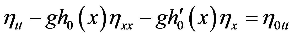 . (7)
. (7)
when  and
and  are given, it is required to determine
  as the solution of (7) subject to the initial condition (4). The horizontal velocity u is then found from (5); for this purpose, we may impose a physically reasonable boundary condition at x = 0, namely
 (8)
(8)
when , q > 0, r > 0, Equation (7) suggests that we consider the solution of the ordinary differential equation
 (9)
(9)
for the determination of .
.
For , the general solution of this equation is [11]
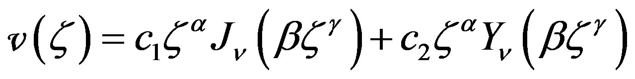 (10)
(10)
where  denote respectively Bessel functions of first and second kind of order
![]() , and
, and
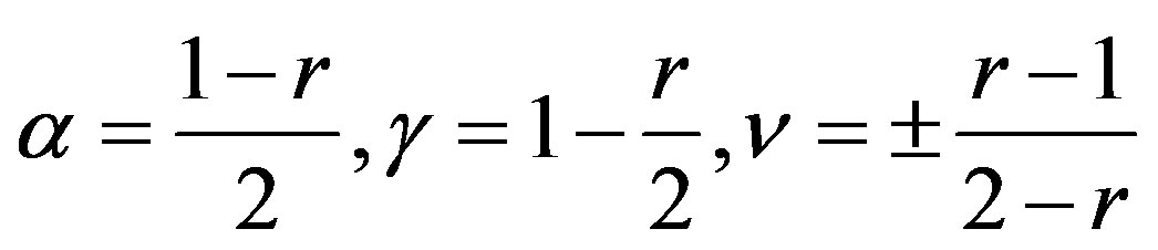 (11)
(11)
For , that is r = 2 the general solution of (9) is
 (12)
(12)
Equations (10) and (12) show that  cannot be both finite at
  (in other words,
  and u cannot be both finite at x = 0 unless
 , and
, and . (13)
To solve the Equation (7) subject to the given initial and boundary conditions, we assume that
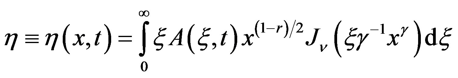 (14)
(14)
Using this in (7), we obtain, by means of (9) and (10), with , the integral equation of first kind
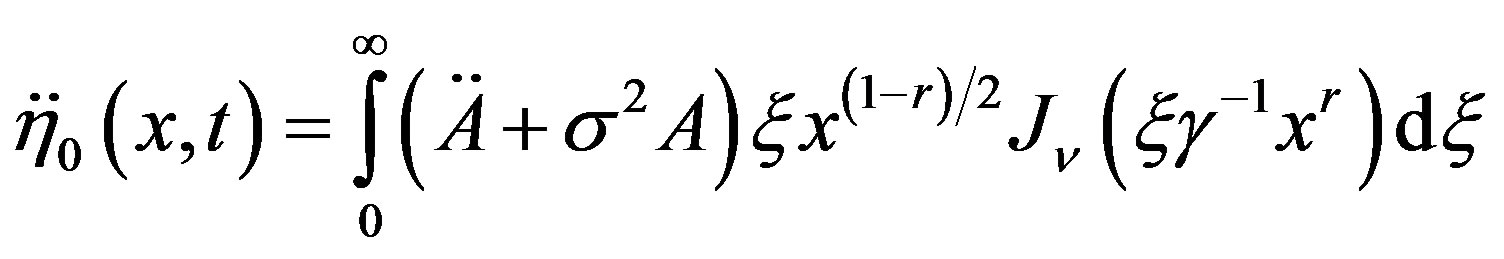 (15)
(15)
where
 (16)
(16)
Then solution of h is obtained with the help of Hankel inversion theorem [12] as
 (17)
(17)
where
 (18)
(18)
where H is the Heaviside unit function.
We note that for r =1 this expression reduces to that of h found for constant slope beach [2].
Taking a time-dependent bottom dislocation like the following
 (19)
(19)
we have been able to evaluate the above integral for all time t with the help of a very nice result [11, p. 58]
 .
.
In the above the t-integral reduces to
where
 Following this evaluation of the t-integral of (17) we spilt the x-integral of (17) in two parts one from x = 0 to
![]() [the first part] which can be evaluated with the help of another result that combines product of two Bessel functions as a terminating hypergeometric series [11, p. 11, 7.2.7 (47)]
[the first part] which can be evaluated with the help of another result that combines product of two Bessel functions as a terminating hypergeometric series [11, p. 11, 7.2.7 (47)]
This spilt corresponds to h11, say, of h which after some tricky manipulation takes a nice form and it corresponds to the free vibration that can be treated as the forerunners. These waves in this spectrum dominate for first few minutes, to be precise for the half period of the quake forcing.
 (20)
(20)
where
and
On the other hand, the second part of x-integral from x = x0 to ¥ contribute h12, say, of h representing the forced wave part is also analytically calculated with its expression being a little complicated is not shown here. We hope to analyze their character in a subsequent paper. At this stage, we remark qualitatively that h12 catch up the free waves beyond half period t and dominate the wave spectrum gradually for t > t.
3. Discussion on the Nature of the Waves with the Help of Some Illustrative Figures
Before we proceed further and discuss the steady-state nature of the waves and the energy transmission let us provide some illustrative figures showing the nature of h11 and h12 in an attempt to distinguish them for small time. We will take for a particular type of bottom dislocation of the following form
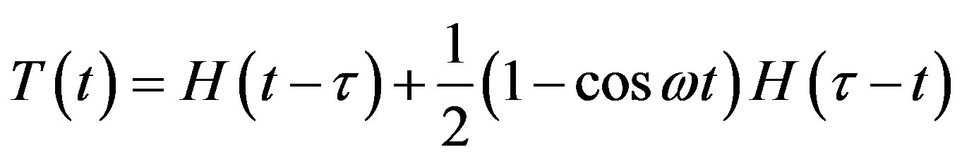
with ,
,  and
and 
The following two figures (Figures 2 and 3) depicting h11 and h12 for small time when r = 0.7 and r = 0.8, that is for two different sloppiness of the ocean bed and in both the cases we find the prominence of h11 over h12 as it was shown analytically and we call this h11 as the forerunners.
The next two graphs (Figures 4 and 5) illustrate nature of h for two different values of r, namely r = 0.7 and r = 0.8,
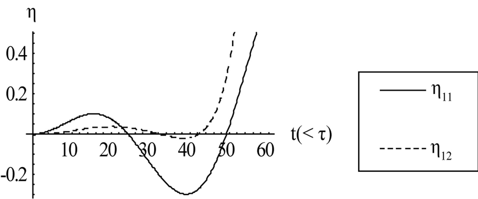
Figure 2. Comparison of h11 and h12 for a particular r = 0.7 and it shows the dominance of h11 when t < t.
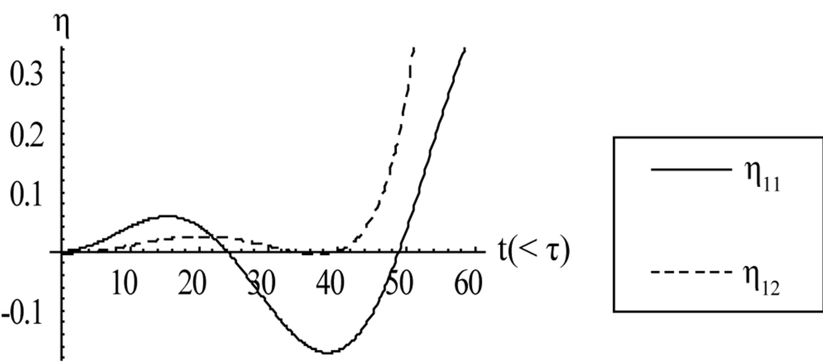
Figure 3. Comparison of h11 and h12 for another r = 0.7 and again the same of dominance of h11 when t < t.
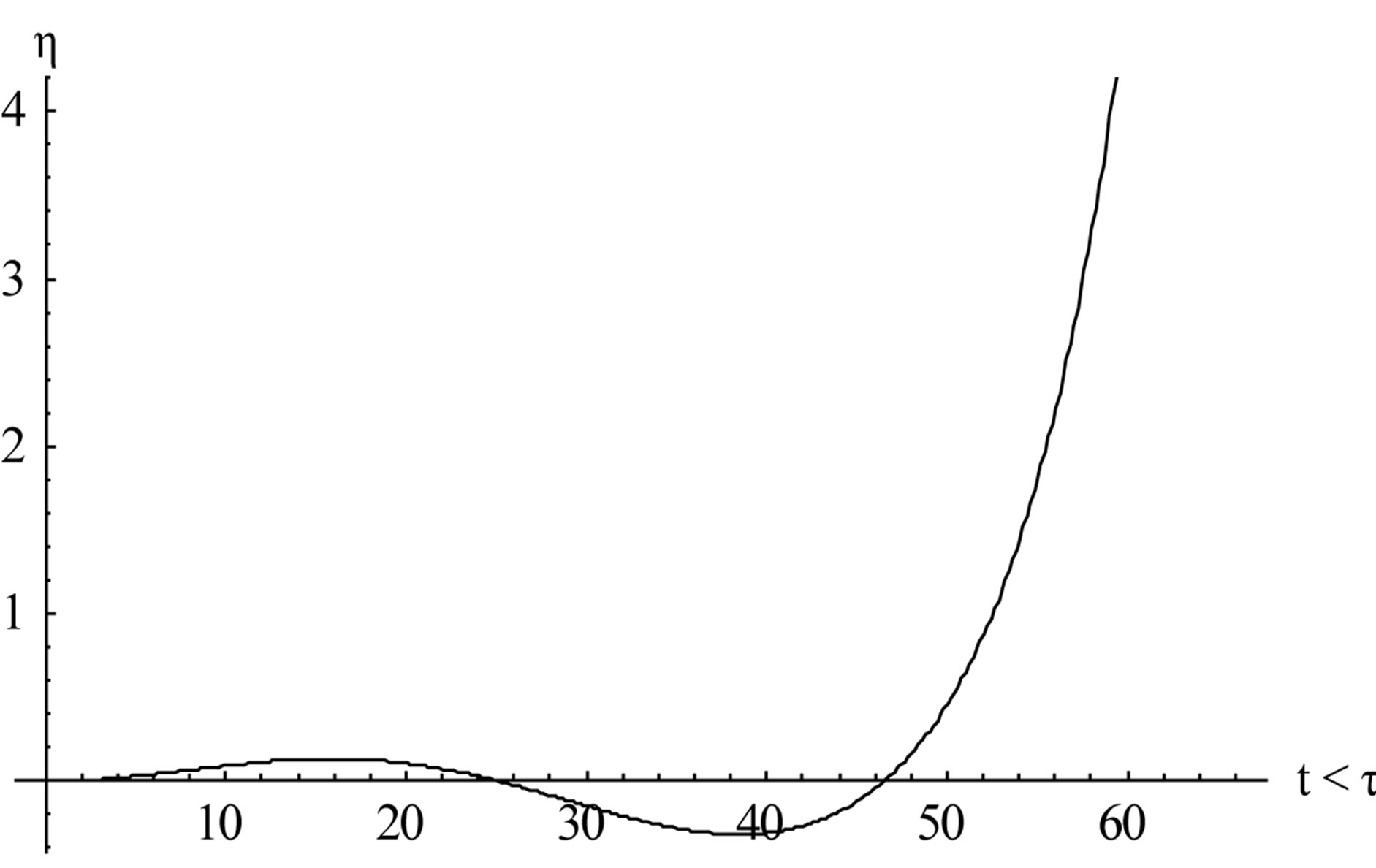
Figure 4. The nature of h for some sloppiness r = 0.7.
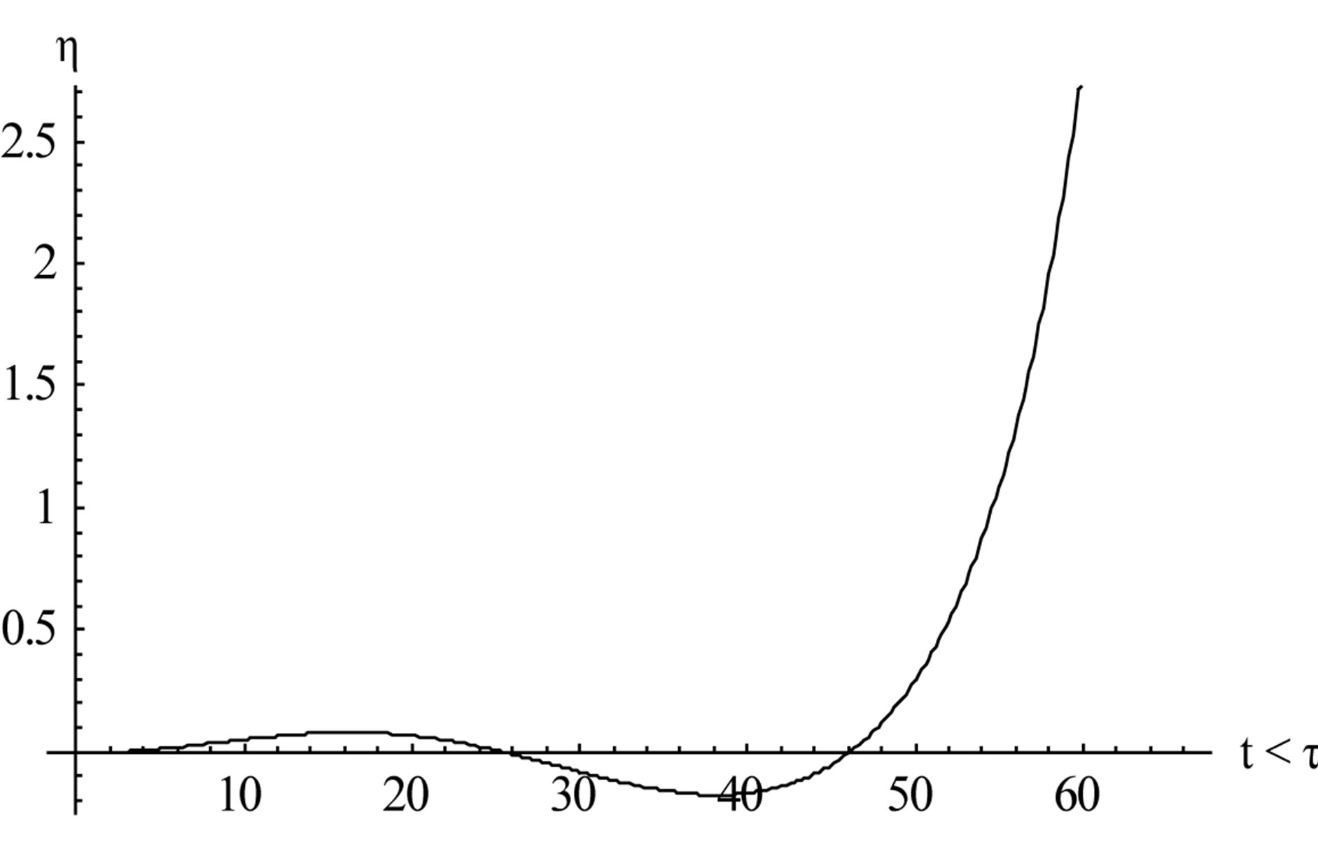
Figure 5. Again the nature of h for some arbitrary sloppiness given by r = 0.8.
here we find h increasing indefinitely with increase of time. Our analytical result also has shown this. It indicates that there might be some sort singularity at t = t, the reason of which may be the sudden disappearance of the bottom vibration at t = t. For any such definite conclusion, though, we require further analytical investigation of the motion for t > t.
The spilt of h namely h12 which comes from the second part of x-integral in (17) while integrating it from x = x0 to ¥ consists of three parts: one of which has a wave form and the other two are standing disturbances, analytical expressions of which is valid for 2/3 < r < 4/3. We restrain ourselves of writing those complicated expressions rather give some illustration of h12 below for two different arbitrary sloppiness of the ocean floor.
The Figures 6 and 7 indicate the nature of h12 in the wave spectrum it actually corresponds to the forced wave part of h which will dominate the spectrum over those which are small and corresponds to the natural frequencies of wave motion.
4. Periodic Ground Motion: Steady-State Solution of ( and u
We assume
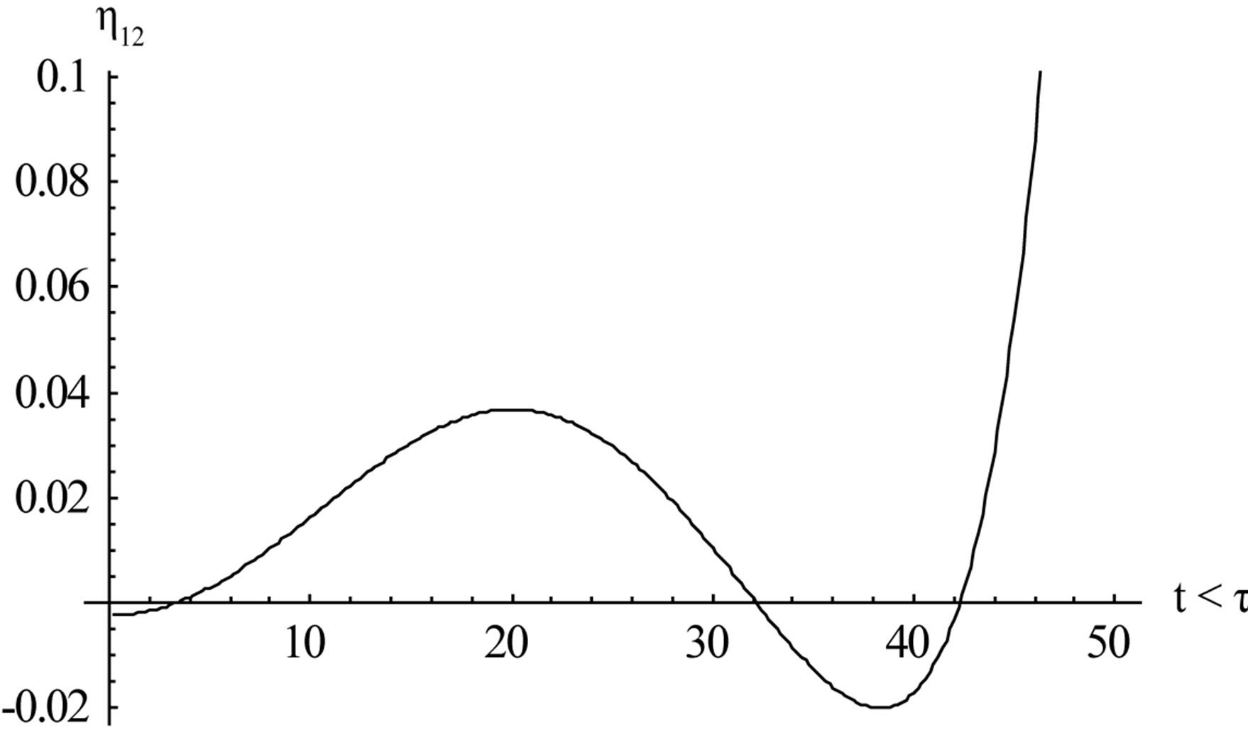
Figure 6. The graph of h12 when t < t, r = 0.7.
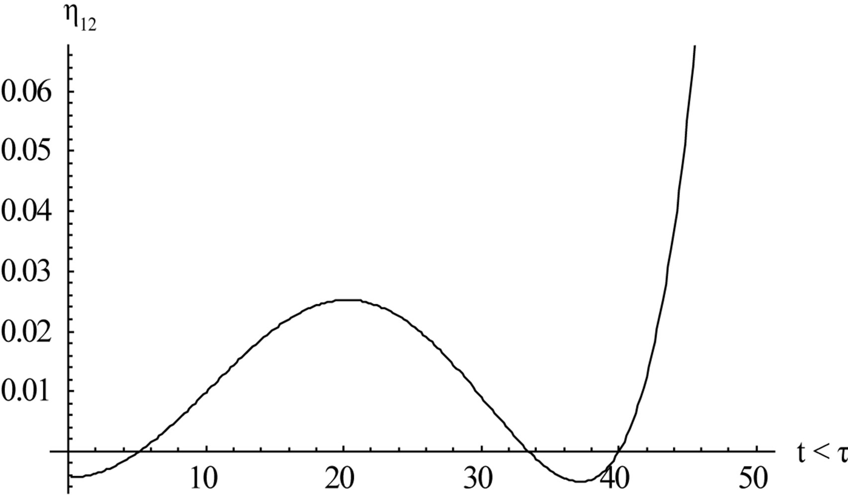
Figure 7. The graph of h12 when t < t, r = 0.8.
 ,
, ;
;
 , t > 0 and show that a steady state
  exists and also determine the corresponding values of
  and u.
Steady-State Value of (
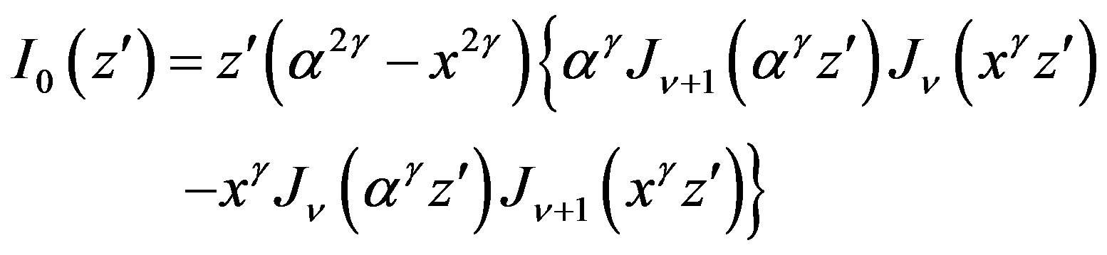
When the integration with respect to s in (17) is completed, we get
 (21)
(21)
where
![]() , (22)
, (22)
 . (23)
We spilt the ![]() -range in (21) into the sub-intervals
-range in (21) into the sub-intervals  and
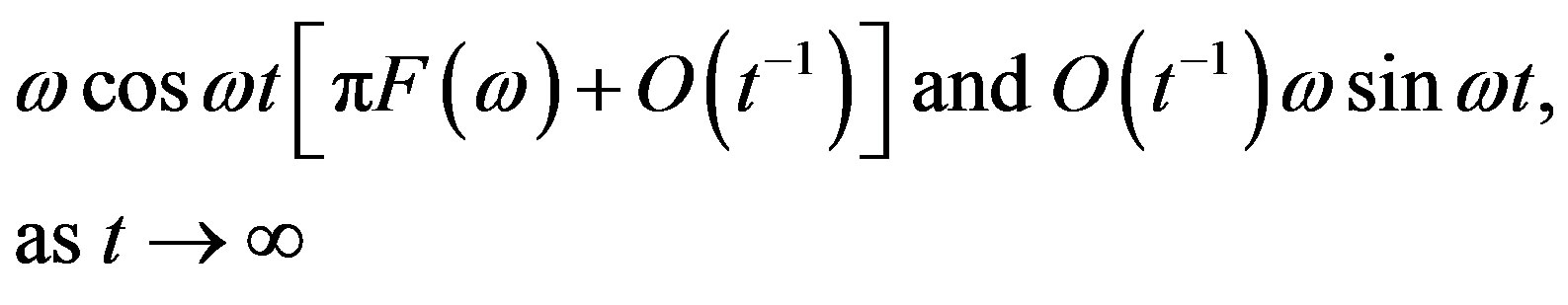
and . By the help of known results on Fourier integrals, the part of the integral in (21) over the interval
  is asymptotically equal to
 (24)
(24)
The remaining part of the integral in (21) is written as
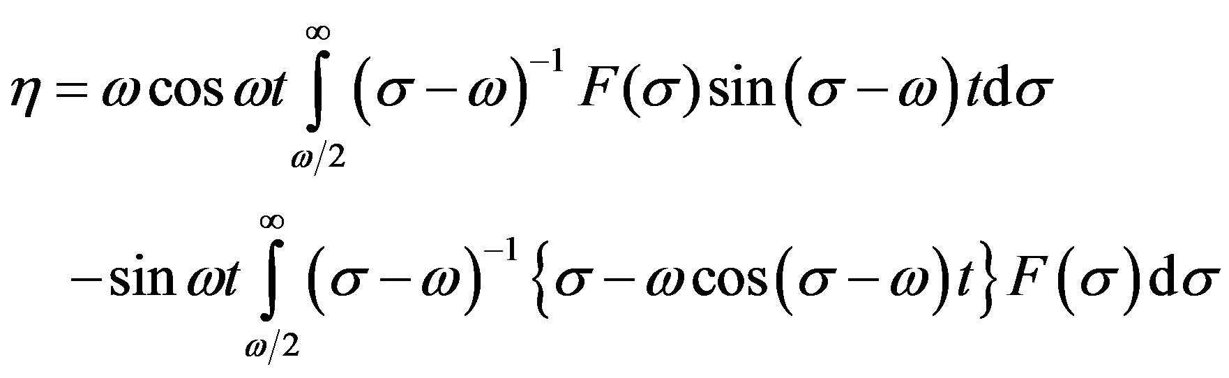 (25)
(25)
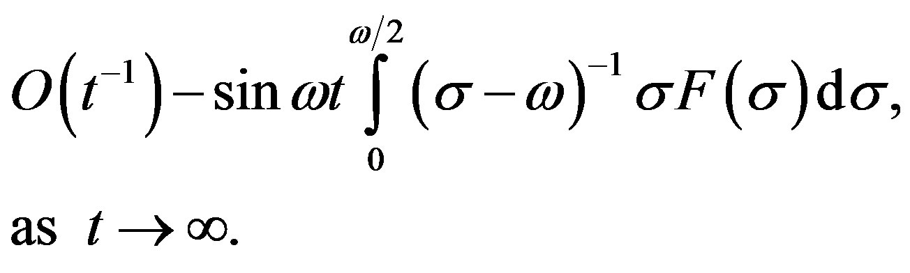
Combining (24) and (25), we get for the integral in (21) the expression
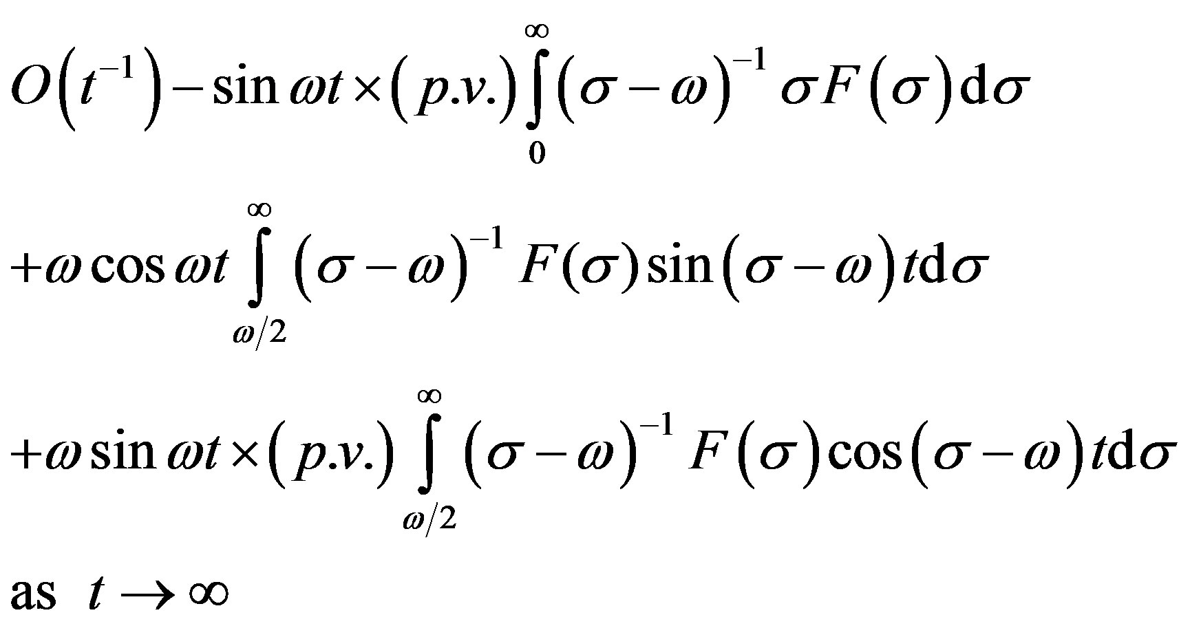 (26)
(26)
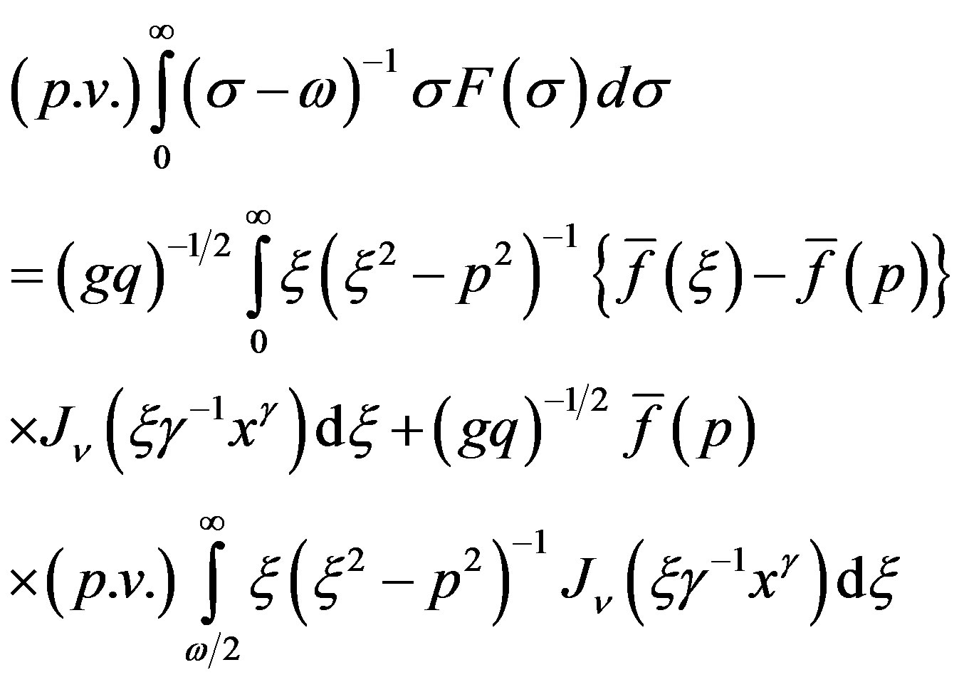
Here the symbol  indicates the Cauchy Principal value of the integral in question. Following Bochner [9], the asymptotic values of the third and fourth terms of (26) are respectively
 (27)
(27)
The results in (27) hold provided 1)  is differentiable with respect to
 ![]() in
in ;
;
2)  exists;
3)  and
and  are each absolutely integrable in
 .
.
Equation (21) then gives
 (21a)
(21a)
Writing , we have
 (21b)
(21b)
By Oberhettinger, F. [13, Section 4.32] the second term is
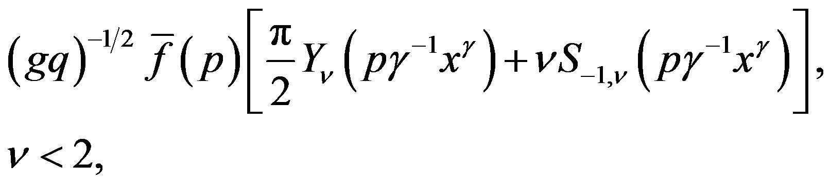 (21c)
(21c)
where  denotes Bessel function of the second kind, and
  is Lommel’s function. We note that since 0 < r < 2 in our discussion,
  imposes the further restriction
 .
.
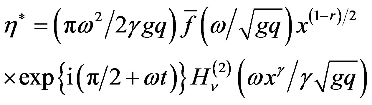
Using the results (21b) and (21c) in (21a), we finally obtain the steady-state value of :
:
 (28)
(28)
For the same periodic ground motion and following the same procedure as described above to obtain , we find the steady-state value of u as
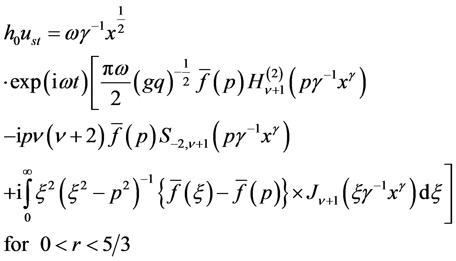 (29)
(29)
Here  denotes Bessel function of the second kind, and
  is Lommel’s function. The first term of both
  and
and , as given below, represent progressive waves:
 (30)
(30)
 (31)
(31)
We also note that h* is an integral of the hyperbolic equation
 (32)
(32)
The rest part of  as well as
  represent clearly standing waves. Since g > 0 in our case, we may use the asymptotic expansion of
  for z ≥ 1 to obtain h* for large x:
 (33)
(33)
The wave described by (28) propagates towards x ® +¥ according to the equation
 (34)
(34)
Thus this wave moves with a variable acceleration unless r = 1 when the acceleration is constant [cp. [2], p. 449]. The height of the wave decreases with the time or distance from the source, according to the factor 
(which is equivalent to ). Since the depth increases as x, this corresponds to Green’s law of shallow water waves.
5. Transmission of Energy
A notable feature of the steady-state solution is that no energy is transmitted through the liquid for frequencies
 which make
 , and hence h* = 0, u*
= 0, the part  and
and  being a standing wave. That these critical frequencies may form a countably infinite set as shown by the following example:
 (35)
(35)
with
 (36)
(36)
Then
 (37)
(37)
The zeros of , for
, for  and x real, are known to be countably infinite. If
  be the n-th position zero of
 , the critical frequencies
  are given by
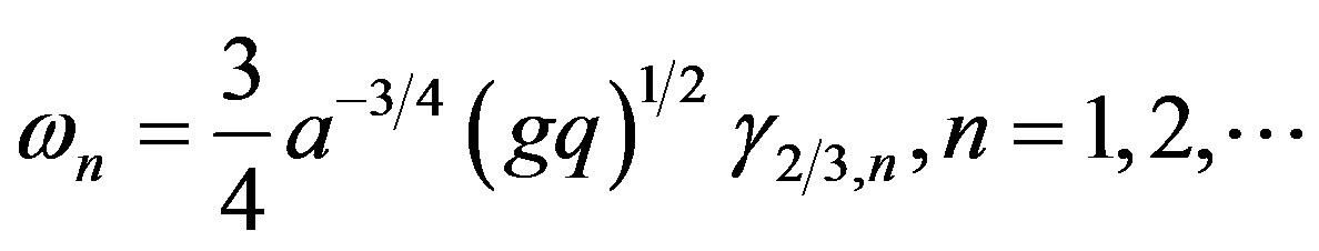 (38)
(38)
6. Conclusion
After the evaluation of s-integral in (17) the splitting of the x-integral in two parts is not arbitrary but instead a necessary one, so the existence of the forerunners. Tsunami forerunners arrive before the arrival of the main tsunami waves with typically smaller amplitude, existence of such waves and a correct analytical expression of which is tried to put up here over a variable sloping beach. Another interesting observation is that the choice of the depth profile , at distance x from the shoreline, makes the dispersive relation [viz. Equation (16)] dispersive while in the classical shallow water theory it is non-dispersive. Leaving aside the actual physical dislocation of the sea floor the solution provided here is correct for all t. In fact if we apply the sea bed deformation due to earthquake as given by Okada’s solution [14] we may perhaps need to employ some numerical work although in that case one has to remain cautious about wave integrals and their oscillatory nature have to be taken into consideration. We know wave is a means of transmission of energy through a medium where the medium itself doesn’t travel. For a progressive wave the transmission of energy takes place which can be described by a simple formula
 , where a = wave amplitude, c = wave velocity. If wave amplitude vanishes for some frequencies of the applied disturbances then the transmission of energy is zero, which has happened here. Needless to mention that the there is no transmission of energy for standing waves. Although we have shown it as a steady-state phenomenon for which there is no transmission of energy into the liquid, we surmise that the result may possibly hold for all time. This implies that some earth quakes may fail to generate propagating waves.
7. Acknowledgements
The author is deeply indebted to Prof. (Retd.) Asim Ranjan Sen, Department of Mathematics, Jadavpur University, Calcutta, India for his help and suggestions during the preparation of this paper. The author is also grateful for the anonymous reviewer for suggesting some improvements which have since been incorporated in the paper.
Some portion of this work was presented by the author at the ISOPE 2012 conference [15] held at Rhodes Island, Greece.
REFERENCES
- C. E. Synolakis and E. N. Bernard, “Tsunami Science before and beyond Boxing Day 2004,” Philosophical Transactions of the Royal Society A, Vol. 364, No. 1845, 2006, pp. 2231-2265. doi:10.1098/rsta.2006.1824
- E. O. Tuck and L. S. Hwang, “Long Wave Generation on a Sloping Beach,” Journal of Fluid Mechanics, Vol. 51, No. 3, 1972, pp. 449-461. doi:10.1017/S0022112072002289
- P. L.-F. Liu, P. Lynett and C. E. Synolakis, “Analytical Solution for Forced Long Waves on a Sloping Beach,” Journal of Fluid Mechanics, Vol. 478, 2003, pp. 101-109. doi:10.1017/S0022112002003385
- U. Kanoglu and C. E. Synolakis, “Long Wave Runup on Piecewise Linear Topographies,” Journal of Fluid Mechanics, Vol. 374, 1998, pp. 1-28.
- C. E. Synolakis, “Tsunami Runup on Steep Slopes: How Good Linear Theory Is,” Natural Hazards, Vol. 4, No. 2- 3, 1991, pp. 221-234. doi:10.1007/BF00162789
- J. J. Stoker, “Water Waves,” Interscience Pulishers, New York, 1957.
- S. Tinti and R. Tonini, “Evolution of Tsunamis Induced by Near-Shore Earthquakes on a Constant Slope Ocean,” Journal of Fluid Mechanics, Vol. 535, 2005, pp. 33-64. doi:10.1017/S0022112005004532
- E. Pelinovsky, T. Talipova, et al., “Nonlinear Mechanism of Tsunami Wave Generation by Atmospheric Disturbances,” Natural Hazards and Earth System Sciences, Vol. 1, 2001, pp. 243-250. doi:10.5194/nhess-1-243-2001
- J. V. Weahausen and E. V. Laitone, “Surface Waves,” In: Handbuch der Physik, Vol. 9, Springer, Berlin, 1960, pp. 446-778.
- B. Edward, “Tsunami an Underrated Hazard,” Cambridge University Press, Cambridge, 2005.
- Erdélyi, et al., “Higher Transcendental Functions,” Vol. 2, McGraw-Hill, New York, 1953, p. 58.
- Erdélyi, et al., “Tables of Integral Transforms,” Vol. 2, McGraw-Hill, New York, 1954, p. 29.
- F. Oberhettinger, “Tables of Bessel Transforms,” Springer, Berlin, 1970.
- Y. Okada, “Internal Deformation Due to Shear and Tensile Faults in a Half-Space,” Bulletin of the Seismological Society of America, Vol. 82, No. 2, 1992, pp. 1018-1040.
- A. Bandyopadhyay, “Mathematical Modeling of Tsunami Waves Generated by Bottom Motion on a Non-Uniformly Sloping Beach,” Proceedings of 22nd ISOPE Conference, Rhodes, June 2012, pp. 68-71.