ABSTRACT

If a non-zero graviton mass exists, the question arises if a release of gravitons, possibly as a “Graviton gas” at the onset of inflation could be an initial vacuum state. Pros and cons to this idea are raised, in part based upon Bose gases. The analysis starts with Volovik’s condensed matter treatment of GR, and ends with consequences, which the author sees, if the supposition is true.

Keywords:

Graviton Gas, Cosmological Vacuum State

1. Introduction

Volovik’s [1] book as of 2003 has a chapter on how a Bose gas can be used to obtain a vacuum energy. We extrapolate from this idea, and link it to what was done by Glinka [2] , as to Wheeler De Witt (WdW) treatment of semi-classical style physics in his boson treatment of a “graviton gas” in order to make a similar analogy to what is done by Park [3] , namely his so called version of a temperature sensitive cosmological constant parameter. Then, afterwards, links of how entropy may be connected with an evolution of the resulting cosmological vacuum energy expression, for a graviton gas are explored.

The authors’ beliefs as to if this hypothesis can be tested will be the final part of the manuscript.

2. Review of the Volovik Model for Bose Gases

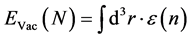
Volovik [1] derives in page 24 of his manuscript a description of a total vacuum energy via an integral over three dimensional space

(1.1)

The integrand to be considered is, using a potential defined by as given by Volovik for weakly interacting Bose gas particles, as well as

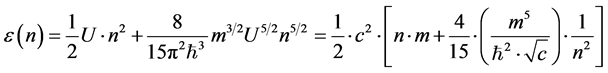(1.2)

For the sake of argument, m, as given above will be called the mass of a graviton, n a numerical count of gravitons in a small region of space, and afterwards, adaptations as to what this expression means in terms of entropy generation will be subsequently raised. A simple graph of the 2^nd term of Equation (1.2) with comparatively large m and with has the following qualitative behavior. Namely for

(1.3)

when n is very small, and as at the onset of inflation.

If we view this as having an indication of when the deviation from usual quantum linearity, the implication is that right at the start of the production of n “gravitons” that there is a cut off right at the start of graviton production, i.e. the implications for ‘tHooft’s [4] non linearity embedding of quantum systems for gravitons would be in that the conditions for non linear embedding are likely in place as a pre cursor to graviton production. What we are observing is right at the start of the production of gravitons, i.e. the moment emergence of graviton states occurs, we have extinguishment of a contribution of classical embedding, but the pre cursor to that would mean graviton production would be initially “framed” by a non linear contribution.

To quantify this, it would be to have with an additional, ‘tHooft [4] style embedding of a usual Q.M. treatment of a spin two particle. In what is stated later about emergence, the author claims that, in analogy to CDW, with emergence of CDW particles, that if there is emergence, that the would be equivalent to the degree of “slope” of a emergent “instanton” and/or instanton- anti instanton structure, which is written in CDW as S-S’. The statement as to emergence, if it occurs is, in both cosmology and CDW given as below, with the caveat that the slope, with its disappearance, in a thin wall representation is for a purely QM treatment of space time emergent particles. The author asserts that a non zero would be given in effect via Figure 3, as a non box like S-S’ pair having ‘tHooft [4] style embedding of emergent QM structure.

An interesting datum to bring up for evaluation. ‘tHooft [4] talked about equivalence classes in his 2002 and 2006 publications. We can then write a wave functional for representing the nucleated states as of Figure 3 as follows. moving from the “floor” of Figure 3, as it rises above, is in sync with moving toward the “thin wall approximation” of minimization of classical contributions to the emergence state, i.e. if Figure 3 were a rectangular block moving upward, with no contributions other than the block itself moving “upward” it would represent a pure “QM” contribution to emergence. Deviations from this block shape represent a non linear semi classical embedding state, with different, continuum of being continuum states and part of ‘tHooft [4] equivalence classes as seen in the CDW wave function below [5]

(1.4)

There exist a “regularization term” we identify with regularization term which will be seen in Equation (1.5) below, and which has a functional dependence in a fashion which will be derived in the future as moves “up” from the “floor” of Figure 3. Also, if we are talking about the beginning of inflation, where would be approximately a constant in time, we can, in the neighborhood of Planck time.

(1.5)

Furthermore, if we take density of this initial state, as given by as far as an information density value at the start of inflation, we get that there is initially a situation for which the regularization term does not contribute right at/just after Planck time

(1.6)

Go to Appendix A as far as a description as to how and why in four dimensions. The links to entropy generation, and actual vacuum state values, will be subsequently raised after elucidating the particulars of a modification of Y.J. Ng’s [6] entropy count hypothesis, brought up by Beckwith in several conferences. The point to raise is the following about a graviton gas. i.e. if the

mass of a graviton is nearly zero, and if the term plays a role,

albeit in nearly a nearly non-existent fashion, for tiny graviton mass, then the existence of this second term is in sync with ‘tHooft’s deterministic quantum mechanics. Volovik calls the 2^nd term a “regularization term”, and its importance can be seen as a way to quantify the affects of an embedding of initial quantum information within a larger structure, which is highly non linear. Doing so would help us determine if with an initial frequency which can be picked up in GW/Graviton detectors. We shall now consider how to model emergent structure as given in Figure 1, Figure 2, and Figure 3.

3. Review of Y. J. Ng’s Entropy Hypothesis

As used by Ng [6]

(1.7)

This, according to Ng [6] , leads to entropy of the limiting value of, if will be modified by having the following done, namely after his use of quantum infinite statistics, as commented upon by Beckwith

(1.8)

Eventually, the author hopes to put on a sound foundation what ‘tHooft [4] is doing with respect to. ‘tHooft [4] deterministic quantum mechanics and equiva-

lence classes embedding quantum particle structures. Our supposition is that the sample space, is extraordinarily small, putting an emphasis upon being quite small, leading to high frequency behavior for the resulting generated N. For extremely small volumes for nucleation of a particle, in initial space, this leads to looking at an inter relationship between a term for initial entropy, of the order of, and if the following expression for detectable frequency, with = initial frequency ~, an initial scale factor, and today’s scale factor behavior, as given by Buoanno [7] is true.

(1.9)

As written up by Buoanno [7] , even if initial frequencies are enormous, the present day frequencies should be, tops of the order of 100 Hz for initial gravitational waves, i.e. the factor, would be almost non-existent. On the other hand, if the embedding structure containing the initial vacuum energy formation has an initially undisturbed character, with minimum breakage of an instanton formation of composite particles, then the frequency would be, instead closer to with an initial frequency ~. We assert that the embedding structure of initial space time would be important to determining if is a datum we can extract, and observe.

4. Conditions to Test for Experimentally to Determine if Exist in the Present Era

As an example we consider a first order phase transition in the early universe. This can lead to a period of turbulent motion in the broken phase fluid, giving rise to a GW signal. Using the results from Durrer [8] .

“If turbulence is generated in the early universe during a first order phase transition, as discussed in the introduction, one has the formation of a cascade of eddies. The largest ones have a period comparable to the time duration of the turbulence itself (of the phase transition).According to Equation (16), these eddies generate GWs which inherit their wavenumber. Smaller eddies instead have much higher frequencies, and one might at first think that they imprint their frequency on the GW spectrum. However, since they are generated by a cascade from the larger eddies, they are correlated and cannot be considered as individual sources of GWs.” We have serious doubts about that last sentence.

Also brought up are GWs produced by the neutrino anisotropic stresses, which generate a turbulent phase. These would be weaker than E and M contributions to anisotropic stresses. For the record as stated in Kojima’s [9] article

Another more familiar example of extra anisotropic stress is that of a primordial magnetic field (PMF). The amplitude of the energy density and magnetic anisotropic stress of the PMF again both scale as radiation density. We doubt that such anisotropic stress would be pertinent to HFGW production. Our supposition is that relic graviton production, not just eddies, as speculated by Durrer also play a role as far as detection, Durrer’s [8] write up exclusively focuses upon eddies, and turbulence in initial GW production.

Wei-Tou Ni [10] in has a very direct statement that DECIGO [11] and Big Bang Observer [12] look for GWs in the higher frequency range, which may give measurements, especially if is not low frequency. Ni also writes, for stochastic backgrounds, that “The minimum detectable intensity of a stochastic GW background”

(1.10)

i.e. Equation (1.9), and the primary difficulty is in accommodating in a sensible fashion. Where is in part analyzed by data brought up by M. Maggiore, [11] . Having said that, then the issue is, are relic conditions for gravitons and GW are linked to entropy, and an initial entropy value of ~10¹⁰. Before saying this, we need to consider the role degrees of freedom, is in the initial phases of inflation.

5. Difficulty in Visualizing What Is in the Initial Phases of Inflation

Secondly, we look for a way to link initial energy states, which may be pertinent to entropy, in a way which permits an increase in entropy from about at the start of the big bang to about to today. One such way to conflate entropy with an initial cosmological constant may be of some help, i.e. if or smaller, i.e. in between the threshold value, and the cube of Planck length, one may be able to look at coming up with an initial value for a cosmological constant as given by as given by [12]

(1.11)

We assert here, that Equation (1.10) is the same order of magnitude as Equation (1.4). To get this, we also look at how to get a suitable value. Then making the following identification of total energy with entropy via looking at models, i.e. consider Park’s model of a cosmological “constant” parameter scaled via background temperature [3]

(1.12)

A linkage between energy and entropy, as seen in the construction, looking at what Kolb [13] put in, i.e.

(1.13)

Here, the idea would be, to make the following equivalence, namely look at,

(1.14)

Note that in the case that quantum effects become highly significant, that the contribution as given by and potentially much smaller, as in the threshold of Planck’s length, going down to possibly as low as 4.22419 × 10⁻¹⁰⁵ m³ = 4.22419 × 10⁻⁹⁶ cm³ leads us to conclude that even with very high temperatures, as an input into the initial entropy, that is very reasonable. Note though that Kolb and Turner [13] , however, have that is at most about 120, whereas the author, in conversation with H. De La Vega [14] , in 2009 indicated that even the exotic theories of have an upper limit of about 1200, and that it is difficult to visualize what is in the initial phases of inflation.

De La Vega [14] stated in Como Italy, that he, as a conservative cosmologist, viewed defining in the initial phases of inflation as impossible. So, then the following formulation of density fluctuations would have to be looked at directly

(1.15)

where we will put in a candidate for the for initial conditions, and then use that as far as answering questions as far as formulating an answer as far as entropy fluctuations, and candidates for density fluctuations, as well as early values of the Hubble parameter. Having such a relatively small value of as placed with

(1.16)

This will lead to comparatively low values for which will be linked to the behavior of a cosmological “constant” parameter value, which subsequently changes in value later, i.e., Equation (1.17) will be for a configuration just before the onset of the big bang itself. Also one can directly write

(1.17)

And, also,

(1.18)

An initially

(1.19)

By conventional cosmological theory, limits of are at the upper limit of 100 - 120, at most, according to Kolb and Turner [13] (1991). is specified for nucleation of a bubble, as a generator of GW. Early universe models with ~ 1000 or so are not in the realm of observational science, yet, according to Hector De La Vega [14] (2009) in personal communications with the author,) at the Colmo, Italy astroparticle physics school, ISAPP, Furthermore, the range of accessible frequencies as given by Equation (1.19) is in sync with

(1.20)

for peak frequencies with values of 10 MHz. The net affect of such thinking is to proclaim that all relic GW are inaccessible. If one looks at Figure, for frequencies as high as up to 10⁶ Hertz, this counters what was declared by Turner and Wilzenk [15] (1990): that inflation will terminate with observable frequencies in the range of 100 or so Hertz. The problem is though, that after several years of LIGO, no one has observed such a GW signal from the early universe, from black holes, or any other source, yet. About the only way one may be able to observe a signal for GW and/or gravitons may be to consider how to obtain a numerical count of gravitons and/or neutrinos for

(1.21)

And this leads to the question of how to account for a possible mass/informa- tion content to the graviton.

6. Break Down of Quark―Gluon Models for Generation of Entropy

It gets worse if one is asserting that there is, in any case, a quark gluon route to determine the role of entropy. To begin this analysis, let us look at what goes wrong in models of the early universe. The assertion made is that this is due to the quark―Gluon model of plasmas having major “counting algorithm” breaks with non counting algorithm conditions, i.e. when plasma physics conditions BEFORE the advent of the Quark gluon plasma existed. Here are some questions which need to be asked.

1) Is QGP strongly coupled or not? Note: Strong coupling is a natural explanation for the small (viscosity) Analogy to the RHIC: J/y survives DE confinement phase transition

2) What is the nature of viscosity in the early universe? What is the standard story? (Hint: AdS-CFT correspondence models). Question 2 comes up since

(1.22)

typically holds for liquid helium and most bosonic matter. However, this relation breaks down. At the beginning of the big bang. As follows i.e. if Gauss- Bonnet gravity is assumed, in order to still keep causality, one needs

This even if one writes for a viscosity over entropy ratio the following

(1.23)

A careful researcher may ask why this is so important. If a causal discontinuity as indicated means the ratio is, or less in value, it puts major restrictions upon viscosity, as well as entropy. A drop in viscosity, which can lead to major deviations from in typical models may be due to more collisions.

Then, more collisions due to WHAT physical process? Recall the argument put up earlier, i.e. the reference to causal discontinuity in four dimensions, and a restriction of information flow to a fifth dimension at the onset of the big bang/ transition from a prior universe? That process of a collision increase may be inherent in the restriction to a fifth dimension, just before the big bang singularity, in four dimensions, of information flow. In fact, it very well be true, that initially, during the process of restriction to a 5^th dimension, right before the big bang,

that. Either the viscosity drops nearly to zero, or else the entropy

density may, partly due to restriction in geometric “sizing” may become effectively nearly infinite. It is due to the following qualifications put in about Quark ? Gluon plasmas which will be put up, here. Namely, more collisions imply less viscosity. More Deflections ALSO implies less viscosity. Finally, the more momentum transport is prevented, the less the viscosity value becomes. Say that a physics researcher is looking at viscosity due to turbulent fields. Also, perturbative calculated viscosities: due to collisions. This has been known as Anomalous Viscosity in plasma physics, (this is going nowhere, from pre-big bang to big bang cosmology). Appendix B gives some more details as far as the

So happens that RHIC models for viscosity assume

(1.24)

As Akazawa [16] noted in an RHIC study, equation 1.80 above makes sense if one has stable temperature T, so that

(1.25)

If the temperature T wildly varies, as it does at the onset of the big bang, this breaks down completely. This development is FRANKLY Mission impossible: AND why we need a different argument for entropy, i.e. Even for the RHIC, and in computational models of the viscosity for closed geometries―what goes wrong in computational models

・ Viscous Stress is NOT µ shear

・ Nonlinear response: impossible to obtain on lattice ( computationally speaking)

・ Bottom line: we DO NOT have a way to even define SHEAR in the vicinity of big bang!!!!

i.e. the quark gluon stage of production of entropy, and its connections to early universe conditions may lead to undefined conditions which, i.e. like shear in the beginning of the universe, cannot be explained. i.e. what does viscosity mean in the neighborhood of time where?

7. Inter Relationship between Graviton Mass and the Problem of a Sufficient Number of Bits of from a Prior Universe, to Preserve Continuity between Fundamental Constants from a Prior to the Present Universe?

V.A. Rubakov and, P.G. Tinyakov [17] gives that there is, with regards to the halo of sub structures in the local Milky Way galaxy an amplitude factor for gravitational waves of

(1.26)

If we use LISA values for the Pulsar Gravitational wave frequencies, this may mean that the massive graviton is ruled out. On the other hand leads to looking at, if

(1.27)

If the radius is of the order of billion light-years ~4300 Mpc or much greater, so then we have, as an example , so then one is getting

(1.28)

This Equation (1.28) is in units where.

If grams per graviton, and 1 electron volt is in rest mass, so. Then [18]

(1.29)

Then, exist

. (1.30)

If each photon, as stated above is grams per photon [19] , then

Initially transmitted photons. (1.31)

Furthermore, if there are, today for a back ground CMBR temperature of 2.7 degrees Kelvin, with a wave length specified as. This is for a numerical density of photons per cubic meter given by

(1.32)

As a rough rule of thumb, if, as given by Weinberg [20] (1972) that early quantum effects, for quantum gravity take place at a temperature Kelvin, then, if there was that temperature for a cubic meter of space, the numerical density would be, roughly times greater than what it is today. Forget it. So what we have to do is to consider a much smaller volume area. If the radii of the volume area is, then we have to work with a de facto initial volume. i.e. the numerical value for the number of photons at, if we have a per unit volume area based upon Planck length, instead of meters, cubed is photons for a cubic area with sides at Kelvin However, initially transmitted photons! Either the minimum distance, i.e. the grid is larger, or Kelvin

8. Finally: What Can be Stated about?

We assert that at a minimum, we can write, the following. Namely that to begin a reasonable inquiry, that

(1.33)

If one has that, the above effect is to put restrictions upon stochastic treatments of for frequencies at or above 10⁶ Hertz. Note here that spectral density is, in some cases allowing for substitution of the spectral density function via the sort of arguments given in Appendix B below.

9. Conclusion. A Graviton Gas Inevitably Has Semi Classical Features. Cosmological Constant Parameter Initially May Be Accounted for via Graviton Release Initially?

The author is fully aware of how Durrer [8] and others use turbulence in early universe conditions, as a way, at the time of the electro weak transition to account for relic graviton production. The electro weak transition, as noted by Rubakov [21] , and others [22] is a candidate for computing the gravity waves induced by anisotropic stresses of stochastic primordial magnetic fields, i.e. a specified magnetic field in the onset of early universe conditions. The author suggests that earlier generation, requiring increased sensitivity of GW detectors, perhaps of may be necessary as to be able to reach higher frequency GW created by graviton production at the onset of inflation. Note that L. Grishchuk [23] , in 2007 specified relic GW production as up to 10 GHz which is far in excess of the values Durrer and others proposal. Indeed, Durrer, Marozzi, and Rinaldi [24] are convinced that any relic conditions for GW must be much lower, with no relic GW observable as they specify it on alleged practical grounds. If one is unable to obtain detector sensitivities of the order of in the foreseeable future, Durrer, Marozzi, and Rinaldi [24] may be right by default. It is worth noting though that physics should be considering if relic GW occurs at all, and the author, and L. Grishchuk [23] have presented mechanisms which may account for their existence in regions of space time evolution well before the electro weak transition, and not necessarily due to conditions linked to anisotropic stress of magnetic fields.

The authors supposition is, in line with what has been presented in the above, that graviton production and early universe entropy production of the order of in initial Planck time seconds may be crucial in formation of an initial graviton gas, which may act like an initial cosmological parameter. The supposition inevitably would be part of the problem of. con-

firming if is possible. Here, Planck tem-

perature = 1.416785(71) × 10³² Kelvin, and the issue would be, if this is true, of giving sufficient reasons for having a scaling argument from initial condition, as specified, of confirming if an analytical proof, backed up by measurements confirms

(1.34)

or 10⁻⁴⁷ GeV⁴, or 10⁻²⁹ g/cm³ or about 10⁻¹²⁰ in reduced Planck units.

I.e. what value of is really needed, so as to obtain 10⁻¹²⁰ today?

If falsifiable experimental measurements for Equation (1.34) may be obtained, the next step would be perhaps in confirming what degree of information exchange such a scaling may imply. The information exchange from a prior to a present universe would be modeled on the template of what would be required, and of what dimensional embedding is needed to do so. Furthermore, what is obtained should be reconciled with an additional constraint which will be put in the next page.

Note that Corda [25] has modeled adiabatically-amplified zero-point fluctuations processes in order to show how the standard inflationary scenario for the early universe can provide a distinctive spectrum of relic gravitational waves. De Laurentis, and Capozziello [26] (2009) have further extended this idea to give a qualified estimate of GW from relic conditions which will be re produced here. Begin with De Laurentis’s idea of a gravitational wave spectrum

(1.35)

is today’s Hubble parameter, while is GW frequency, and is the red shift value of when the universe became matter dominated, i.e. red shift z = 1.55 with an estimated age of 3.5 Giga year, or larger, would be a good starting point, i.e. this is for larger than 3.5 Giga years for when matter domination became most prominent, i.e. the further back goes the larger the upper bound for frequency. The upper range for appears to be about 100 Hertz. Needless to state, though, if drifted to a value of then the upper bound to Hertz. And, we suggest that Hz, if is set higher, i.e., which should be investigated.

We at the close refer the readers to Appendix C for crucial considerations as to the emergence of gravitational astronomy as this relates to a summary as to how to confirm the models so referenced in this paper, as to work by Corda, and the LIGO GW team which is of potentially revolutionary import as far as observational astronomy confirming these ideas so presented.

Acknowledgements

The author thanks Dr. Raymond Weiss, of MIT as of his interaction in explaining Advanced LIGO technology for the detection of GW for frequencies beyond 1000 Hertz and technology issues with the author in ADM 50, November 7^th 2009. Dr. Fangyu Li, of Chongqing University is thanked for lending his personal notes to give substance to the content of page 10 of this document.

This work is supported in part by National Nature Science Foundation of China grant No. 11375279.

Cite this paper

Beckwith, A.W. (2017) Analyzing If a Graviton Gas Acts Like a Cosmological Vacuum State and “Cosmological” Constant Parameter. Journal of High Energy Physics, Gravitation and Cosmology, 3, 388-413. https://doi.org/10.4236/jhepgc.2017.32032

References

Appendix A: Looking at Situations When the Mass of a Graviton is not Zero

A1: Linkage of DM to gravitons and gravitational waves?

Let us state that the object of early universe GW astronomy would be to begin with confirmation of whether or not relic GW were obtainable, and then from there to ascertain is there is linkage which can be made to DM production ... Durrer, Massimiliano Rinaldi [24] (2009), state that there would be probably negligible for this case (practically non-existent) graviton production in cosmological eras after the big bang.. In fact, they state that they investigate the creation of massless particles in a Universe which transits from a radiation- dominated era to any other (via an) expansion law. “We calculate in detail the generation of gravitons during the transition to a matter dominated era. We show that the resulting gravitons generated in the standard radiation/matter transition are negligible” This indicated to the author, Beckwith that it is appropriate to look at the onset of relic GW/Graviton production. One of the way to delineating the evolution of GW is the super adiabatic approximation, done for when as given by M. Giovannini [27] (page 138), when is a solution to

. (A.1)

Which to first order when leads to a GW solution

(A.2)

This will be contrasted with a very similar evolution equation for gravitons, of (i.e. KK gravitons in higher dimensions)

(A.3)

One of the models of linkage between gravitons, and DM is the KK graviton, i.e. as a DM candidate. KK gravitons. Note that usual Randal Sundrum brane theory has a production rate of as the number of Kaluza Klein gravitons per unit time per unit volume Note this production rate is for a formula assuming mass for which T_* > M_X, and that we are assuming that the temperature. Furthermore, we also are looking at total production rate of KK gravitons of the form

(A.4)

where R is the assumed higher dimension ‘size’ and, d is the number of dimensions above 4, and typically we obtain. I.e. we can typically assume tiny higher dimensional ‘dimensions’, very high temperatures, and also a wave length for the resulting KK graviton for a DM candidate looking like

(A.5)

If KK gravitons have the same wavelength as DM, this will support Jack Ng’s treatment of DM. All that needs to put this on firmer ground will be to make a de facto linkage of KK Gravitons, as a DM candidate, and more traditional treatments of gravitons, which would assume a steady drop in temperature from, to eventually much lower temperature scales. Note that in a time interval based as proportional to the inverse of the Hubble parameter, we have the total numerical density of KK gravitons (on a brane?) as

, where give or take an order of magnitude. This number density needs to be fully reconciled to and can be conflated with the dimensionality ‘radius’ value

centimeters for dimensions above 4 space time GR values, with

this value of R being unmanageable for d < 2. V.A. Rubakov [21] and others also (2002) makes the claim of the KK graviton obeying the general Yukawa style potential

(A.6)

As well as being related to an overall wave functional which can be derived from a line element

(A.7)

With (suppressing the u, v coefficients). This evolu-

tion equation for the KK gravitons is very similar to work done by Baumann, Daniel, Ichiki, Kiyotomo, Steinhardt, Paul J. Takahashi, Keitaro [28] (2007) with similar assumptions, with the result that KK gravitons are a linear combination of Bessel functions. Note that one has for gravitons.

(A.8)

Ruth Gregory, Valery A. Ruvakov and Sergei M. Sibiryakov [29] (2000) make the additional claim that for large z ( the higher dimensions get significant) that there are marked oscillatory behaviors, i.e. Rapid oscillations as one goes into the space for branes for massive graviton expansion.

(A.9)

This is similar to what Baumann, Ichiki, Steinhardt, and Takahashi [28] (2007) for GW, in a relic setting, with the one difference being that the representation for a graviton is in the z ( additional dimension) space, as opposed to what Bauman et al. [28] did for their evolution of GW, with an emphasis upon generation in overall GR space time.. Furthermore, the equation given in

for massive graviton evolution as KK gravitons along

dS branes is similar to evolution of GW in more standard cosmology that the author, Beckwith, thinks that the main challenge in clarifying this picture will be in defining the relationship of dS geometry, in overall Randall Sundrum brane world to that of standard 4 space,. We need though, now to look at whether or not higher dimensions are even relevant to GR itself.

A2: How DM would be influenced by gravitons, in 4 dimensions

We will also discuss the inter relationship of structure of DM, with challenges to Gaussianity. The formula as given by

(A.10)

Will be gone into. The variation, so alluded to which we will link to a statement about the relative contribution of Gaussianity, via looking at the gravitational potential

(A.11)

Here the expression variations from Gaussianity, while the statements as to what contributes, or does not contribute will be stated in our presentation. Furthermore, is a linear Gaussian potential, and the overall gravitational potential is altered by inputs from the term, presented,. The author discussed inputs into variations from Gaussianity, which were admittedly done from a highly theoretical perspective with Sabino Matarre [30] on July 10, with his contributions to non Guassianity being constricted to a reported range of, as given to Matarre [30] , by Senatore, et al [31] , 2009. The author, Beckwith, prefers a narrower range along the lines of. Needless to state, though, dealing with what we can and cannot measure, what is ascertained as far as DM, via a density profile variation needs to have it reconciled with DM detection values

(A.12)

It is note worthy to note that the question of DM/KK gravitons, and also the mass of the graviton not only has relevance to whether or not, higher dimensions are necessary/advisable in space time models, but also may be relevant to if massive gravitons may solve/partly fulfill the DE puzzle. To whit, \KK gravitons would have a combined sum of Bessel equations as a wave functional representation. In fact V. A Rubakov [21] (2002) writes that KK graviton representation as,

after using the following normalization,

where are different forms of Bessel functions, to obtain the KK graviton/ DM candidate representation along RS dS brane world

(A.13)

This allegedly is for KK gravitons having an order of TeV magnitude mass (i.e. for mass values at 0.5 TeV to above a TeV in value) on a negative tension RS brane. What would be useful would be managing to relate this KK graviton, which is moving with a speed proportional to with regards to the

negative tension brane with as a possible initial starting value for the KK graviton mass, before the KK graviton, as a ‘massive’ graviton moves with velocity along the RS dS brane. If so, and if represents an initial state, then one may relate the

mass of the KK graviton, moving at high speed, with the initial rest mass of the graviton, which in four space in a rest mass configuration would have a mass many times lower in value, i.e. of at least, as opposed to. Whatever the range of the graviton mass, it may be a way to make sense of what was presented by Dubovsky, Flauger, Starobinsky, and Thackev [32] (2009) who argue for graviton mass using CMBR measurements, of up to. This can be conflated with M. Alves, O. Miranda, and J de Araujo’s [33] results arguing that non zero graviton mass may lead to acceleration of our present universe, in a manner usually conflated with DE, i.e. their graviton mass would be about grams, leading to a possible explanation for when the universe accelerated, i.e. the de-acceleration parameter, due to changes in the scale factor, written as

Appendix B. Next Generation GW Detectors

The following section is to improve upon the range of GW detected, as can be presented below. We use Figure 4 as given explicitly below

The relation between and the spectrum is often expressed as written by L. P. Grishchuk, (2001) [35] , as

(B.1)

The curve of the pre-big-bang models shows that of the relic GWs is almost constant from 10 Hz to 10¹⁰ Hz. of the cosmic string models is about 10⁻⁸ in the region 1 Hz to 10¹⁰ Hz; its peak value region is about 10⁻⁷ - 10⁻⁶ Hz. The reason for this section is to deal with the statement made by Buoanno [7] (2006) that the following limit is verbatim, and cannot be improved upon if one looks at BBN, the following upper bound should be considered:

(B.2)

Here, Buoanno [7] is using, and a reference from Kosowoky, Mack, and Kahniashhvili [36] (2002) as well as Jenet et al. [37] (2006). Using this upper bound, if one insist upon assuming, as Buoanno [7] (2006) does, that the frequency today depends upon the relation

(B.3)

The problem in this is that the ratio, assumes that is “today’s” scale factor. In fact, using this estimate, Buoanno [7] comes up with a peak frequency value for relic/\early universe values of the electroweak era-generated GW graviton production of

(B.4)

By conventional cosmological theory, limits of as given by Kolb and Turner [13] (1991) are at the upper limit of 100 - 120. In addition according to Kolb and Turner [13] (1991), is specified for nucleation of a bubble, as a generator of GW. Early universe models with ~ 1000 or so are not in the realm of observational science, yet, according to Hector De La Vega [14] (2009) in personal communications with the author, at the Colmo, Italy astroparticle physics school, ISAPP. All the assumptions above lead to a de facto limit of, which is what Dr. Fangyu Li [38] disputes: The following notes are also in response to a referee quote which Fangyu answered the following query, which is re produced

Quote:

“The most serious is that a background strain at 10 GHz corresponds to a (total) which violates the baryon nuclei-synthesis epoch limit for either GWs or EMWs. (Total) needs to be smaller than 10⁻⁵ otherwise the cosmological Helium/hydrogen abundance in the universe would be strongly affected ...”

The answer, which the author copied from Dr. Li, i.e., If, then Dr. Li claims

(B.5)

The following is Dr. Fangyu Li’s argument as given to the author in personal notes:

1) LIGO and our coupling electromagnetic system [39] [40] in the free space are different detecting schemes for GWs. LIGO detects shrinking and extension of interferometer legs, this is a displacement effect. The CEMS detects the perturbative photon fluxes, this is a parameter perturbation effect of the EM fields. Although their sensitivities all are limited by relative quantum limits, concrete mechanisms of the quantum limits are quite different.

2) The minimal detectable amplitude of LIGO depends on [41]

(B.6)

where L is the interferometer length. Because detecting band of LIGO is limited in ~1 Hz - 1000 Hz, this is a very strong constraint for h_min. Thus, h_min of LIGO is about ~10⁻²³ - 10⁻²⁴ in this band.

3) The minimal detectable amplitude of cavity depends on arguments similar to the ones brought up in reference [42] as well as the following formulation

(B.7)

For the constant-amplitude HFGWs, and

(B.8)

for the stochastic relic HFGWs and considerations which were given to the author in a discussion he had with Dr. Weiss of MIT [15] .

Because Q factor of superconducting cavity in the low-temperature condition can reach up to ~10¹⁰ - 10¹², if we assume Q = 10¹¹, , B = 3T (coupling static magnetic field to the cavity), V = 1 m³, then

(B.9)

for the constant-amplitude HFGW.

and

(B.10)

for the stochastic relic HFGW.

4) The CEMS [40] is that

The minimal detectable amplitude h depends on the relative standard quantum limit (SQL) (G.V. Stephenson 2008, 2009), [42]

(B.11)

for the stochastic relic HFGW, is the total EM energy of the system. For the typical parameters: B = 3 T, L = 6 m. signal accumulation time, P = 10 W (the power of Gaussian Beam-GB), even if the fractal membranes are absent (using natural decay rate of the GB in the radial direction), then equivalent Q factor (Notice, here Q factor is different from cavity’s Q factor) can reach up to 10³¹, then

. (B.12)

If we use fractal membranes, even if a conservative estimation, we have

. (B.13)

Equation (B.11) is similar to Equation (B.6) and Equation (B.7). An important difference is that in the cavity case, while there is no limitation of the maximum accumulation time of the signal in the CEMS, but only minimal accumulation time of the signal. Thus, the sensitivity in the CEMS is the photon signal limited, not quantum noise limited.

5) LIGO and our scheme have quite different detecting mechanisms (the displacement effect and the EM parameter perturbation effect) and detecting bands (~1 Hz - 1000 Hz and 1 GHz ~ 10 GHz), their comparison should not be only the amplitude of GWs, but also the energy flux of GWs. In fact, the energy flux of any weak GW is proportional to. Thus, the CEMS with sensitivity h = 10⁻³⁰, and the LIGO with sensitivity h = 10⁻²², correspond to the GWs of the same energy flux density. This means that the EM detection schemes with the sensitivity of h = 10⁻³⁰, (or better) GHz-10 GHz in the future should not be surprise.

The SQL is a basic limitation. Any useful means and advanced models might give better sensitivity, but there is no change of order of magnitude in the SQL range. For example, if we use squeezed quantum states for a concrete detector, then the sensitivity would be improved 2 - 3 times than when the squeezed quantum state is absent in the detector, but it cannot improve one order of magnitude or more According to more accepted by the general astrophysics community values as told to the author by Dr. Weiss [41] , the estimate, for the upper limit of F on relic GWs should be smaller than, while recent data analysis (B.P. Abbott et al., (2009)) [34] shows the upper limit of, as in Figure 4 should be. By using such parameters, Dr. Li estimates the spectrum and the RMS amplitude. The relation between and the spectrum is often expressed as (L. P. Grishchuk) [35] ,

(B.14)

so

(B.15)

where, the present value of the Hubble frequency. From Equation (B.14) and Equation (3.15)), we have

(a)

If, then, (B.16)

If, then, (B.17)

(b)

, H = 10⁻³¹, then, (B.18)

If, then (B.19)

Such values of, would be essential to ascertain the possibility of detection of GW from relic conditions, whereas, as data collected and binned to be summed over different frequencies as given by

with the integral numerical summed up value, weighted of binned data sets to make the following identification [18] .

(B.20)

Furthermore, the numerical summed up value of binned data sets, in each frequency f value is [18]

(B.21)

Equation (1.23) is for a very narrow range of frequencies, that to first approximation, make a linkage between an integral representation of and. Note also that Dr. Li suggests, as an optimal upper frequency to investigate, then

, (B.22)

and

(B.23)

Thus an obvious gap still exists between the theoretical estimation and detecting reality, but there are large rooms to advance and improve the CEMS. These are upper values of the spectrum, and should be considered as preliminary. Needed in this mix of calculations would be a way to ascertain a set of input values for into a formula for. The objective is to get a set of measurements to confirm if possible the utility of using, experimentally (in order to ascertain, experimentally, a relationship between gravitational wave energy density, and numerical count of gravitons at a given frequency f) the numerical count of up to a value of having [18]

. If there is roughly a 1-1 correspondence between gravitons and neutrios (highly unlikely), then. [28] counting the number of gravitons per cell space should also consider what Buoanno [7] wrote, for Les Houches if one looks at BBN, the following upper bound should be considered:

(B.24)

Here, Buoanno [7] is using, does, that the frequency today depends upon the relation

(B.25)

The problem in this is that the ratio, assumes that is “today’s” scale factor. In fact, using this estimate, Buoanno [7] comes up with a peak frequency value for relic/\early universe values of the electroweak era-generated GW graviton production of

(B.26)

By conventional cosmological theory, limits of are at the upper limit of 100 - 120, at most, according to Kolb and Turner [13] (1991). is specified for nucleation of a bubble, as a generator of GW. Early universe models with ~ 1000 or so are not in the realm of observational science, yet, according to Hector De La Vega [14] (2009) in personal communications with the author, at the Colmo, Italy astroparticle physics school, ISAPP, Furthermore, the range of accessible frequencies as given by Equation (B.26) is in sync with for peak frequencies with values of 10 MHz. The net affect of such thinking is to rule out examining early universe gravitons as measurable and to state as a way of to rule out being able to measure relic GW and gravitons, via the premise that all relic GW are inaccessible. If one looks at Figure 4, for frequencies as high as up to 10⁶ Hertz, this counters what was declared by Turner and Wilzenk [43] (1990): that inflation will terminate with observable frequencies in the range of 100 or so Hertz. The problem is though, that after several years of LIGO, no one has observed such a GW signal from the early universe, from black holes, or any other source, yet. About the only way one may be able to observe a signal for GW and/or gravitons may be to consider how to obtain a numerical count of gravitons and/or neutrinos for [41]

. And this leads to the question of how to account for a possible mass/ information content to the graviton.

Appendix C. Crucially Important Developments as of 2016 Which Impact the Observability of Some of the Phenomena Discussed in This Document

Abbot et al., in [43] outlined the crucial physics of gravitational waves, and this should be a way of either falsifying or confirmation of the essential details of Equation (B.26) of Appendix B. I.e. nothing should contradict the basics of GW predictions as given in [43] . In addition, it is important to note that not only is Equation (B.26) to be confirmed or to be falsified, but that the details of [43] plus other work should be used to confirm and get falsifiable criterion to establish if General relativity is the final gravitational theory for Gravitation, but if we have to consider Scalar-Tensor gravity as is gone into great detail in [44] by Corda. The details in Appendix A and Appendix B could prove decisively important as to this matter. Finally, a subsequent analysis of the event GW150914 in [45] put in a limit of 10 to the 13 kilometers as far as a lower bound to gravitational physics, and by extension affected massive gravity theories significantly. [45] is also linked to Equation (B.26) of Appendix B and is of decisive theoretical import too.

Submit or recommend next manuscript to SCIRP and we will provide best service for you:

Accepting pre-submission inquiries through Email, Facebook, LinkedIn, Twitter, etc.

A wide selection of journals (inclusive of 9 subjects, more than 200 journals)

Providing 24-hour high-quality service

User-friendly online submission system

Fair and swift peer-review system

Efficient typesetting and proofreading procedure

Display of the result of downloads and visits, as well as the number of cited articles

Maximum dissemination of your research work

Submit your manuscript at: http://papersubmission.scirp.org/

Or contact jhepgc@scirp.org

References

- 1. Volovik, G. (2003) The Universe in a Helium Droplet. International Series of Monographs on Physics 117, Oxford University Press, Oxford.
- 2. Glinka, L. (2007) Quantum Information from Graviton-Matter Gas. Symmetry, Integrability and Geometry: Methods and Applications, 3, 087. https://doi.org/10.3842/sigma.2007.087
- 3. Park, D., Kim, H. and Tamarayan, S. (2002) Nonvanishing Cosmological Constant of Flat Universe in Brane-World Scenario. Physics Letters B, 535, 5-10. https://doi.org/10.1016/S0370-2693(02)01729-X
- 4. ‘T Hooft, G. (2002) Determinism Beneath Quantum Mechanics. http://arxiv.org/PS_cache/quant-ph/pdf/0212/0212095v1.pdf
- 5. Beckwith, A.W. (2006) A New S-S’ Pair Creation Rate Expression Improving upon Zener Curves for I-E Plots. Modern Physics Letters B, 20, 849-861. http://arxiv.org/abs/math-ph/0411045 https://doi.org/10.1142/S0217984906011219
- 6. Ng, Y.J. (2007) Holographic Foam, Dark Energy and Infinite Statistics. Physics Letters B, 657, 10-14. https://doi.org/10.1016/j.physletb.2007.09.052
Ng, Y.J. (2008) Spacetime Foam: From Entropy and Holography to Infinite Statistics and Nonlocality. Entropy, 10, 441-461.
https://doi.org/10.3390/e10040441 - 7. Buonanno, A. (2006) Gravitational Waves. In: Bernardeau, F., Grojean, C. and Dalibard, J., Eds., Particle Physics and Cosmology: The Fabric of Space-Time, Elsevier, Amsterdam, 10-52.
- 8. Durrer, R. (2006) On the Frequency of Gravitational Waves. http://theory.physics.unige.ch/~durrer/papers/freq.pdf
- 9. Kojima, K. (2010) Generation of Curvature Perturbations with Extra Anisotropic Stress. http://arxiv.org/PS_cache/arxiv/pdf/0910/0910.1976v2.pdf
- 10. Ni, W.-T. (2009) Direct Detection of the Primordial Inflationary Gravitational Waves. International Journal of Modern Physics D, 18, 2195-2199. http://arxiv.org/pdf/0905.2508 https://doi.org/10.1142/s0218271809016041
- 11. Maggiore, M. (2000) Stochastic Backgrounds of Gravitational Waves. arXiv:gr-qc/0008027v1 Maggiore, M. (2000) Gravitational Wave Experiments and Early Universe Cosmology. Physics Reports, 331, 283-367. https://doi.org/10.1016/S0370-1573(99)00102-7
- 12. Padmanabhan, T. (2008) From Gravitons to Gravity: Myths and Reality. International Journal of Modern Physics D, 17, 367-398. gr-qc/0409089 https://doi.org/10.1142/S0218271808012085
Padmanabhan, T. (2006) An Invitation to Astrophysics. World Scientific Series in Astronomy and Astrophysics 8, World Scientific, Singapore. - 13. Kolb, E. and Turner, S. (1994) The Early Universe. Westview Press, Chicago.
- 14. Dicussion with De La Vega, H., at Villa Olmo, Como, Italy July 11 2009. ISAPP.
- 15. Turner, M.S. and Wilzenk, F. (1990) Relic Gravitational Waves and Extended Inflation. Physical Review Letters, 65, 3080-3083. https://doi.org/10.1103/PhysRevLett.65.3080
- 16. Asakawa, M., Bass, S. and Müller, B. (2006) Anomalous Viscosity of an Expanding Quark-Gluon Plasma. Physical Review Letters, 96, Article ID: 252301.
https://doi.org/10.1103/physrevlett.96.252301
Asakawa, M., Hatsuda, T. and Nakahara, Y. (2001) Maximum Entropy Analysis of the Spectral Functions in Lattice QCD. Progress in Particle and Nuclear Physics, 46, 459-508.
https://doi.org/10.1016/S0146-6410(01)00150-8 - 17. Rubakov, V.A. and Tinyakov, P.G. (2008) Infrared-Modified Gravities and Massive Gravitons. Physics-Uspekh, 51, 759-792. http://ufn.ru/en/articles/2008/8/a/references.html https://doi.org/10.1070/PU2008v051n08ABEH006600
- 18. Beckwith, A. (2010) Applications of Euclidian Snyder Geometry to the Foundations of Space Time Physics. http://vixra.org/abs/0912.0012
- 19. Honig, W. (1974) A Minimum Photon “Rest Mass”—Using Planck’s Constant and Discontinuous Electromagnetic Waves. Foundations of Physics, 4, 367-380. https://doi.org/10.1007/BF00708542
- 20. Weinberg, S. (1972) Gravitation and Cosmology: Principles and Applications of the General Theory of Relativity.
- 21. Rubakov, V. (2002) Classical Theory of Gauge Fields. Princeton University Press, Princeton.
- 22. Caprini, C. and Durrer, R. (2001) Gravitational Wave Production: A Strong Constraint on Primordial Magnetic Fields. Physical Review D, 65, Article ID: 023517. https://doi.org/10.1103/PhysRevD.65.023517
- 23. Grishchuk, L. (2008) Discovering Relic Gravitational Waves in Cosmic Microwave Background Radiation. http://arxiv.org/abs/0707.3319
- 24. Durrer, R., Marozzi, G. and Rinaldi, M. (2009) On Adiabatic Renormalization of Inflationary Perturbations. Physical Review D, 80, Article ID: 065024. http://arxiv.org/abs/0906.4772 https://doi.org/10.1103/physrevd.80.065024
- 25. Corda, C. (2007) Analysis of the Transverse Effect of Einstein’s Gravitational Waves. International Journal of Modern Physics A, 22, 4859-4881. http://adsabs.harvard.edu/abs/2007arXiv0707.1943C https://doi.org/10.1142/S0217751X07037172
- 26. De Laurentis, M. and Capozziello, S. (2009) Stochastic Background of Relic Scalar Gravitational Waves tuned by Extended Gravity. Nuclear Physics B—Proceedings Supplements, 194, 212-217. http://arxiv.org/abs/0906.3689 https://doi.org/10.1016/j.nuclphysbps.2009.07.025
- 27. Giovannini, M. (2008) A Primer on the Physics of the Cosmic Microwave Background. World Press Scientific, Singapore. https://doi.org/10.1142/6730
- 28. Baumann, D., Ichiki, K., Steinhardt, P. and Takahashi, K. (2007) Physical Review D, 76, Article ID: 084019. http://arxiv.org/abs/hep-th/0703290 https://doi.org/10.1103/PhysRevD.76.084019
- 29. Gregory, R., Ruvakov, V. and Sibiryakov, S. (2000) Opening up Extra Dimensions at Ultra-Large Scales. Physical Review Letters, 84, 5928-5931. https://doi.org/10.1103/PhysRevLett.84.5928
- 30. Matarre, S., at Villa Olmo, Como, Italy July 11 2009. ISAPP.
- 31. Senatore, L., Tassev, S. and Zaldarriaga, M. (2009) Cosmological Perturbations at Second Order and Recombination Perturbed. Journal of Cosmology and Astroparticle Physics, No. 08, 031. http://iopscience.iop.org/1475-7516/2009/08/031 https://doi.org/10.1088/1475-7516/2009/08/031
- 32. Dubovsky, S., Flauger, R., Starobinsky, A. and Tkachev, I. (2009) Signatures of a Graviton Mass in the Cosmic Microwave Background. Report UTTG-06-09, TCC-23-09. http://arxiv.org/abs/0907.1658
- 33. Alves, M., Miranda, O. and de Araujo, J. (2009) Can Massive Gravitons be an Alternative to Dark Energy? arXiv: 0907.5190
- 34. Abbott, B.P., et al. (2009) An Upper Limit on the Stochastic Gravitational-Wave Background of Cosmological Origin. Nature, 460, 990-993. https://doi.org/10.1038/nature08278
- 35. Grishchuk, L.P. (2001) Relic Gravitational Waves and Their Detection. Lecture Notes in Physics, 562, 167-194. https://doi.org/10.1007/3-540-40988-2_9
- 36. Kosowsky, A., Mack, A. and Kahniashvili, T. (2002) Gravitational Radiation from Cosmological Turbulence. Physical Review D, 66, Article ID: 024030. https://doi.org/10.1103/physrevd.66.024030
- 37. Jenet, F.A., Hobbs, G.B., van Straten, W., Manchester, R.N., Bailes, M., Verbiest, J.P.W., Edwards, R.T., Hotan, A.W., Sarkissian, J.M. and Ord, S.M. (2006) Upper Bounds on the Low-Frequency Stochastic Gravitational Wave Background from Pulsar Timing Observations: Current Limits and Future Prospects. Astrophysical Journal, 653, 1571-1576. http://iopscience.iop.org/0004-637X/653/2/1571 https://doi.org/10.1086/508702
- 38. Personal Notes Delivered to Dr. Beckwith by Dr. Li, Reproduced with His Permission.
- 39. Li, F., Baker, R., Fang, Z., Stephenson, G. and Chen, Z. (2008) Perturbative Photon Fluxes Generated by High-Frequency Gravitational Waves and Their Physical Effects. European Physical Journal C, 56, 407-423. https://doi.org/10.1140/epjc/s10052-008-0656-9
- 40. Li, F., Yang, N., Fang, Z., Baker, R., Stephenson, G. and Wen, H. (2009) Signal Photon Flux and Background Noise in a Coupling Electromagnetic Detecting System for High Frequency Gravitational Waves. Physical Review D, 80, Article ID: 064013. https://doi.org/10.1103/PhysRevD.80.064013
- 41. Weiss, R. (2009) Personal Communications with Author. ADM 50, College Station.
- 42. Stephenson, G.V. (2009) The Standard Quantum Limit for the Li-Baker HFGW Detector. Proceedings of the Space, Propulsion and Energy Sciences International Forum, Huntsville, 24-27 February 2009, 542-547. https://doi.org/10.1063/1.3115563
- 43. Abbott, B.P., et al. (2016) Observation of Gravitational Waves from a Binary Black Hole Merger. Physical Review Letters, 116, Article ID: 061102. https://physics.aps.org/featured-article-pdf/10.1103/PhysRevLett.116.061102 https://doi.org/10.1103/physrevlett.116.061102
- 44. Corda, C. (2009) Interferometric Detection of Gravitational Waves: The Definitive Test for General Relativity. International Journal of Modern Physics D, 18, 2275-2282. arXiv:0905.2502 https://doi.org/10.1142/s0218271809015904
- 45. Abbot, B.P., et al. (2016) Tests of General Relativity with GW150914. Physical Review Letters, 116, Article ID: 221101. https://doi.org/10.1103/physrevlett.116.221101