Mixed-Model U-Shaped Assembly Line Balancing Problems with Coincidence Memetic Algorithm

doi:10.4236/jsea.2010.34040

Paper Menu >>

Journal Menu >>

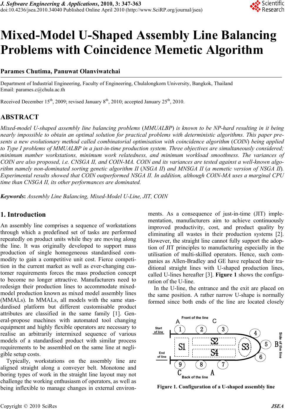J. Software Engineering & Applications, 2010, 3: 347-363

doi:10.4236/jsea.2010.34040 Published Online April 2010 (http://www.SciRP.org/journal/jsea)

347

Mixed-Model U-Shaped Assem bly Line Bal ancin g

Problems with Coincidence Memetic Algorithm

Parames Chutima, Panuwat Olanviwatchai

Department of Industrial Engineering, Faculty of Engineering, Chulalongkorn University, Bangkok, Thailand

Email: parames.c@chula.ac.th

Received December 15th, 2009; revised January 8th, 2010; accepted January 25th, 20 10.

ABSTRACT

Mixed-model U-shaped assembly line balancing problems (MMUALBP ) is known to be NP-hard resulting in it being

nearly impossible to obtain an optimal solution for practical problems with deterministic algorithms. This paper pre-

sents a new evolutionary method called combinatorial optimisation with coincidence algorithm (COIN) being applied

to Type I problems of MMUALBP in a just-in-time production system. Three objectives are simultaneously considered;

minimum number workstations, minimum work relatedness, and minimum workload smoothness. The variances of

COIN are also proposed, i.e. CNSGA II, and COIN-MA. COIN and its variances are tested against a well -known algo-

rithm namely non-dominated sorting genetic algorithm II (NSGA II) and MNSGA II (a memetic version of NSGA II).

Experimental results showed that COIN outperformed NSGA II. In addition, although COIN-MA uses a marginal CPU

time than CNSGA II, its other performances are dominated.

Keywords: Assembly Line Balancing, Mixed-Model U-Line, JIT, COIN

1. Introduction

An assembly line comprises a sequence of workstations

through which a predefined set of tasks are performed

repeatedly on product units while they are moving along

the line. It was originally developed to support mass

production of single homogeneous standardised com-

modity to gain a competitive unit cost. Fierce competi-

tion in the current market as well as ever-changing cus-

tomer requirements forces the mass production concept

to become no longer attractive. Manufacturers need to

redesign their production lines to accommodate mixed-

model production known as mixed model assembly lines

(MMALs). In MMALs, all models with the same stan-

dardised platform but different customisable product

attributes are classified in the same family [1]. Gen-

eral-propose machines with automated tool changing

equipment and highly flexible operators are necessary to

realise an arbitrarily intermixed sequence of various

models of a standardised product with similar process

requirements to be assembled on the same line at negli-

gible setup costs.

Typically, workstations on the assembly line are

aligned straight along a conveyer belt. Monotone and

boring types of work in the straight line layout may not

challenge the working enthusiasm of operators, as well as

being inflexible to manage changes in external environ-

ments. As a consequence of just-in-time (JIT) imple-

mentation, manufacturers aim to achieve continuously

improved productivity, cost, and product quality by

eliminating all wastes in their production systems [2].

However, the straight line cannot fully support the adop-

tion of JIT principles to manufacturing especially in the

utilisation of multi-skilled operators. Hence, such com-

panies as Allen-Bradley and GE have replaced their tra-

ditional straight lines with U-shaped production lines,

called U-lines hereafter [3]. Fig ure 1 shows the configu-

ration of the U-line.

In the U-line, the entrance and the exit are placed on

the same position. A rather narrow U-shape is normally

formed since both ends of the line are located closely

S1 S2

S4 S3

1234

789

Start

of line

End

of line

Front of the line

Back of the line

Side of the line

Figure 1. Configuration of a U-shaped assembly line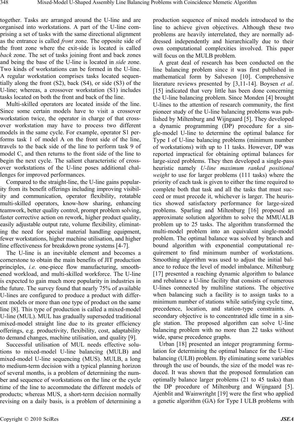

Mixed-Model U-Shaped Assembly Line Balancing Problems with Coincidence Memetic Algorithm

348

together. Tasks are arranged around the U-line and are

organised into workstations. A part of the U-line com-

prising a set of tasks w ith the same directional alignment

as the entrance is called front zone. The opposite side of

the front zone where the exit-side is located is called

back zone. The set of tasks joining front and back zones

and being the base of the U-line is located in side zone.

Two kinds of workstations can be formed in the U-line.

A regular workstation comprises tasks located sequen-

tially along the front (S2), back (S4), or side (S3) of the

U-line; whereas, a crossover workstation (S1) includes

tasks located on both the front and back of the line.

Multi-skilled operators are located inside of the line.

Since some certain models have to visit a crossover

workstation twice, the operator in charge of that cross-

over workstation may have to process two different

models in the same cycle. For example, operator S1 per-

forms task 1 of model A on the front side of the line,

travels to the back side of the line to perform task 9 of

model C, and then returns to the front side of the line to

begin the next cycle. The salient characteristic of cross-

over workstations of the U-line poses additional chal-

lenges for improved performances.

Compared to the straight-line, the U-line gains popular-

ity from its benefit offerings including improving visibil-

ity and communication, operator flexibility, rotatable

mul ti -skilled operators, know-how sharing, enhancing

teamwork, better quality control, prompt problem solving,

faster corrective action on rework, higher product quality,

easily adjustable output rate, volume flexibility, eliminat-

ing the need for special material handling equipment,

fewer workstations, higher machine utilisation, and higher

line effectiveness for breakdown prone systems [4-7].

The U-line is an inevitable element and becomes a

cornerstone to obtain the main benefits of JIT production

principles, i.e. one-piece flow manufacturing, smooth-

ened workload, and multi-skilled workforce. The U-line

is expected to gain much more popularity in industries in

the future. The survey found that nearly 75% of available

U-lines are configured to produce a product with differ-

ent models or more than one type of product on the same

line [8]. This type of production is called a mixed-model

U-line (MUL). MUL has gradually superseded traditional

mixed-model straight line due to its greater efficiency

offerings, e.g. productivity, flexibility, cost, adaptability

to demand changes, machine utilisation, and quality [9].

Successful utilisation of MUL needs effective solu-

tions to mixed-model U-line balancing (MULB) and

mixed-model U-line sequencing (MUS). MULB, a long

to medium-term decision with a typical planning horizon

of several months, is a problem of determining the num-

ber and sequence of workstations on the line or the cycle

time of the line to accommodate the different models of

products; whereas MUS, a short-term decision normally

revising on a daily basis, is a problem of determining a

production sequence of mixed models introduced to the

line to achieve given objectives. Although these two

problems are heavily interrelated, they are normally ad-

dressed independently and hierarchically due to their

own computational complexities involved. This paper

will focus on the MULB problem.

A great deal of research has been conducted on the

line balancing problem since it was first published in

mathematical form by Salveson [10]. Comprehensive

literature reviews presented by [3,11-14]. Boysen et al.

[15] indicated that very little has been done concerning

the U-line balancing problem. Since Monden [4] brought

U-lines to the attention of research community, the first

pioneer study of the U-line balancing problems was pub-

lished by Miltenburg and Wijngaard [5]. They developed

a dynamic programming (DP) procedure for a sin-

gle-model U-line to determine the optimal balance for

Type I of U-line balancing problems (minimum number

of workstations) with up to 11 tasks. However, DP was

reported impractical for obtaining optimal balances for

large-sized problems. They then developed a single-pass

heuristic namely U-line maximum ranked positional

weight to use for larger problems (111 tasks) where the

priority of each task is given to either the time required to

complete both that task and all the tasks that must suc-

ceed or must precede it, whichever is larger. The heuris-

tics showed satisfactory performance for large-sized

problems. Sparling and Miltenburg [16] proposed an

approximate solution algorithm to solve the MMUALB

problem up to 25 tasks. The algorithm transformed the

mul ti-model problem into an equivalent single-model

problem. The optimal balance was solved by branch and

bound algorithm with exponential computational re-

quirement to find minimum number of workstations.

Smoothing algorithm was used to adjust the initial bal-

ance to reduce the level of model imbalance. Miltenburg

[17] presented a reaching dynamic algorithm to balance

and rebalance a U-line facility that consists of numerous

U-lines connected by multiline stations. The objective

when balancing such a facility is to assign tasks to a

minimum number of stations wh ile satisfying cycle time,

precedence, location, and station-type constraints. A

secondary objective is to concentrated idle time in a sin-

gle station. The proposed algorithm can solve U-line

balancing problem with no more than 22 tasks without

wide, sparse precedence graphs.

Urban [18] presented an integer programming formu-

lation for determining the optimal balance for the U-line

balancing (ULB) problem. By eliminating some variables

through the use of bounds, the size of the model was re-

duced. It was shown that the proposed formulation can

optimally balance larger problems (21 to 45 tasks) than

the DP procedure of Miltenburg and Wijngaard [5].

Ajenblit and W ainwritght [19] were the first who applied

a genetic algorithm (GA) for Type I ULB problems with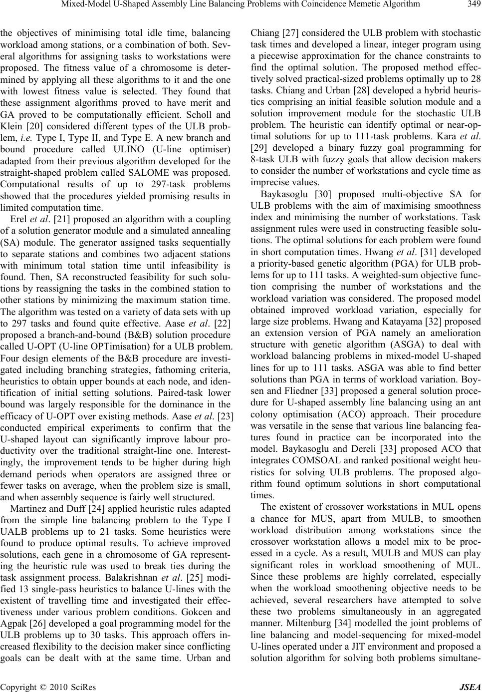

Mixed-Model U-Shaped Assembly Line Balancing Problems with Coincidence Memetic Algorithm

349

the objectives of minimising total idle time, balancing

workload among stations, or a combination of both. Sev-

eral algorithms for assigning tasks to workstations were

proposed. The fitness value of a chromosome is deter-

mined by applying all these algorithms to it and the one

with lowest fitness value is selected. They found that

these assignment algorithms proved to have merit and

GA proved to be computationally efficient. Scholl and

Klein [20] considered different types of the ULB prob-

lem, i.e. Type I, Type II, and Type E. A new bra nch and

bound procedure called ULINO (U-line optimiser)

adapted from their previous algorithm developed for the

straight-shaped problem called SALOME was proposed.

Computational results of up to 297-task problems

showed that the procedures yielded promising results in

limited computation time.

Erel et al. [21] proposed an algorithm with a coupling

of a solution generator module and a simulated annealing

(SA) module. The generator assigned tasks sequentially

to separate stations and combines two adjacent stations

with minimum total station time until infeasibility is

found. Then, SA reconstructed feasibility for such solu-

tions by reassigning the tasks in the combined station to

other stations by minimizing the maximum station time.

The algorithm was tested on a variety of d ata sets w ith up

to 297 tasks and found quite effective. Aase et al. [22]

proposed a branch-and-bound (B&B) solution procedure

called U-OPT (U-line OPTimisation) for a ULB problem.

Four design elements of the B&B procedure are investi-

gated including branching strategies, fathoming criteria,

heuristics to obtain upper bounds at each node, and iden-

tification of initial setting solutions. Paired-task lower

bound was largely responsible for the dominance in the

efficacy of U-OPT over existing methods. Aase et al. [23]

conducted empirical experiments to confirm that the

U-shaped layout can significantly improve labour pro-

ductivity over the traditional straight-line one. Interest-

ingly, the improvement tends to be higher during high

demand periods when operators are assigned three or

fewer tasks on average, when the problem size is small,

and when assembly sequence is fairly well structured.

Martinez and Duff [24] applied heuristic rules adapted

from the simple line balancing problem to the Type I

UALB problems up to 21 tasks. Some heuristics were

found to produce optimal results. To achieve improved

solutions, each gene in a chromosome of GA represent-

ing the heuristic rule was used to break ties during the

task assignment process. Balakrishnan et al. [25] modi-

fied 13 single-pass heuristics to balance U-lines with the

existent of travelling time and investigated their effec-

tiveness under various problem conditions. Gokcen and

Agpak [26] developed a goal programming model for the

ULB problems up to 30 tasks. This approach offers in-

creased flexibility to the decision maker since conflicting

goals can be dealt with at the same time. Urban and

Chiang [27] considered the ULB problem with stochastic

task times and developed a linear, integer program using

a piecewise approximation for the chance constraints to

find the optimal solution. The proposed method effec-

tively solved practical -sized problems optimally u p to 28

tasks. Chiang and Urban [28] developed a hybrid heuris-

tics comprising an initial feasible solution module and a

solution improvement module for the stochastic ULB

problem. The heuristic can identify optimal or near-op-

timal solutions for up to 111-task problems. Kara et al.

[29] developed a binary fuzzy goal programming for

8-task ULB with fuzzy goals that allow decision makers

to consider the number of workstations and cycle time as

imprecise values.

Baykasoglu [30] proposed multi-objective SA for

ULB problems with the aim of maximising smoothness

index and minimising the number of workstations. Task

assignment rules were used in constructing feasible solu-

tions. The optimal solutions for each problem were found

in short computation times. Hwang et al. [31] developed

a priority-based genetic algorithm (PGA) for ULB prob-

lems for up to 111 tasks. A weighted-sum objective func-

tion comprising the number of workstations and the

workload variation was considered. The proposed model

obtained improved workload variation, especially for

large size problems. Hwang and Katayama [32] proposed

an extension version of PGA namely an amelioration

structure with genetic algorithm (ASGA) to deal with

workload balancing problems in mixed-model U-shaped

lines for up to 111 tasks. ASGA was able to find better

solutions than PGA in terms of workload variation. Boy-

sen and Fliedner [33] proposed a general solution proce-

dure for U-shaped assembly line balancing using an ant

colony optimisation (ACO) approach. Their procedure

was versatile in the sense that various line balancing fea-

tures found in practice can be incorporated into the

model. Baykasoglu and Dereli [33] proposed ACO that

integrates COMSOAL and ranked positional weight heu-

ristics for solving ULB problems. The proposed algo-

rithm found optimum solutions in short computational

time s.

The existent of crossover workstations in MUL opens

a chance for MUS, apart from MULB, to smoothen

workload distribution among workstations since the

crossover workstation allows a model mix to be proc-

essed in a cycle. As a result, MULB and MUS can play

significant roles in workload smoothening of MUL.

Since these problems are highly correlated, especially

when the workload smoothening objective needs to be

achieved, several researchers have attempted to solve

these two problems simultaneously in an aggregated

manner. Miltenburg [34] modelled the joint problems of

line balancing and model-sequencing for mixed-model

U-lines operated under a JIT environment and proposed a

solution algorithm for solving both problems simultane-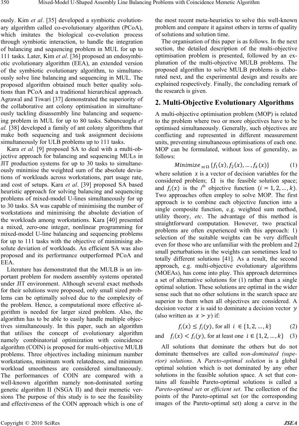

Mixed-Model U-Shaped Assembly Line Balancing Problems with Coincidence Memetic Algorithm

350

ously. Kim et al. [35] developed a symbiotic evolution-

ary algorithm called co-evolutionary algorithm (PCoA),

which imitates the biological co-evolution process

through symbiotic interaction, to handle the integration

of balancing and sequencing problem in MUL for up to

111 tasks. Later, Kim et al. [36] proposed an endosymbi-

otic evolutionary algorithm (EEA), an extended version

of the symbiotic evolutionary algorithm, to simultane-

ously solve line balancing and sequencing in MUL. The

proposed algorithm obtained much better quality solu-

tions than PCoA and a traditional hierarchical approach.

Agrawal and Tiwari [37] demonstrated the superiority of

the collaborative ant colony optimisation in simultane-

ously tackling disassembly line balancing and sequenc-

ing problem in MUL for up to 80 tasks. Sabuncuoglu et

al. [38] developed a family of ant colony algorithms that

make both sequencing and task assignment decisions

simultane ous ly for ULB p roblems up to 111 tasks.

Kara et al. [9] proposed SA to deal with a multi-ob-

jective approach for balancing and sequencing MULs in

JIT production systems for up to 30 tasks to simultane-

ously minimise the weighted sum of the absolute devia-

tions of workloads across workstations, part usage rate,

and cost of setups. Kara et al. [39] proposed SA based

heuristic approach for solving balancing and sequencing

problems of mixed-model U-lines simultaneously for up

to 30 tasks. SA was capable of minimising the number of

workstations and minimising the absolute deviation of

the workloads among workstations. Kara [40] presented

a mixed, zero-one integer, nonlinear programming for

mixed-model U-line balancing and sequencing problems

for up to 111 tasks with the objective of minimising ab-

solute deviation of workloads. An efficient SA was also

proposed and its performance outperformed PCoA and

EEA.

Literature has demonstrated that the MULB is an im-

portant problem for modern assembly systems operated

under JIT environment. Although several exact methods

for their solutions were proposed, only small sized prob-

lems can be optimally solved due to the complexity of

the problem. Hence, a computational more effective al-

gorithm is needed for larger sized problem. Also, the

algorithm has to be able to easily handle multiple objec-

tives simultaneously. In this paper, such an algorithm

that utilises the concept of evolutionary algorithm

namely combinatorial optimization with coincidence

algorithm (COIN) is proposed for multi-objectiv e MULB

problems. Three objectives including minimum number

workstations, minimum work relatedness, and minimum

workload smoothness are considered simultaneously.

The performances of COIN are compared with a

well-known algorithm namely non-dominated sorting

genetic algorithm II (NSGA II) and their memetic ver-

sions The purpose of this study is to see the feasibility

and effectiveness of the COIN approach which is one of

the most recent meta-heuristics to solve this well-known

problem and compare it against others in terms of quality

of solutions and solution time.

The organisation of this paper is as follows. In the next

section, the detailed description of the multi-objective

optimisation problem is presented, followed by an ex-

planation of the multi-objective MULB problems. The

proposed algorithm to solve MULB problems is elabo-

rated next, and the experimental design and results are

explained respectively. Finally, th e concluding remark of

the research is given.

2. Multi-Objective Evolutionary Algorithms

A multi-objective optimisation p roblem (MOP) is related

to the problem where two or more objectives have to be

optimised simultaneously. Generally, such objectives are

conflicting and represented in different measurement

units, preventing simultaneous optimisation s of each on e.

MOP can be formulated, without loss of generality, as

follows:

 Ω {1(),2(),…,()} (1)

where solution  is a vector of decision variables for the

considered problem;

Ω

is the feasible solution space;

and () is the ith objective function (=1, 2, … , ).

Two approaches often employ to solve MOP. The first

approach is to combine each objective function into a

single composite function, e.g. weighted sum method,

utility theory, etc. The advantage of this method is

straightforward computation. However, two practical

problems are often experienced with this approach: 1)

selection of the suitable weights can be very difficult

even for those who are unfamiliar with the problem and 2)

small perturbations in the weights can sometimes lead to

totally different solutions [41]. As a result, the second

approach, e.g. multi-objective evolutionary algorithms

(MOEAs), has come into play. This approach determines

a set of alternative solutions for (1) rather than a single

optimal solution. These solutions are optimal in the wider

sense such that no other solutions in the search space are

superior to them when all objectives are considered. A

decision vector  is said to dominate a decision vector 

(also written as ) if:

()(), for all  {1, 2, … , } (2)

and ()<(), for at least one {1, 2, … , } (3)

All solutions that dominate the others but do not

dominate themselves are called non-dominated (supe-

rior) solutions. A Pareto-optimal solution is a global

optimal solution which is not dominated by any other

solutions in the feasible solution space. A set that con-

tains all feasible Pareto-optimal solutions is called a

Pareto-optimal set or efficient set. The collection of the

points of the Pareto-optimal set (or the corresponding

images of the Pareto-optimal set) along a curve in the

Mixed-Model U-Shaped Assembly Line Balancing Problems with Coincidence Memetic Algorithm

351

objective space that has a set of attributes collectively

dominating all other points not on the frontier are termed

the Pareto-optimal frontier (front) or efficient frontier

(front). An example of the Pareto-optimal solutions for a

two-objective minimisation problem is illustrated in

Figure 2. It is obvious that an amount of sacrifice in one

objective is always incurred to achieve a certain amount

of gain in the other (inverse relationship) while moving

from one Pareto-optimal solution to another. Providing

Pareto-optimal solutions to the decision maker is more

preferable to a single solution since practically, when

considering real-life problems, a final decision is always

based on a trade-off between conflicting objective func-

tions.

MOEAs have recently become popular and have been

applied to a wide range of problems from social to engi-

neering problems [42]. In general, MOEAs are ideally

suited to MOP because they are capable of searching a

whole set of multiple Par eto-optimal solutions in a single

run. In addition, the shape or continuity of the

Pareto-optimal frontier has less effect to MOEAs than

traditional mathematical programming. The approxima-

tion of a true Pareto-optimal set involves two conflicting

objectives: 1.) the distance to the tru e Pareto frontier is to

be minimised, and 2.) the diversity of the evolved solu-

tions is to be maxi mised [43]. To achieve the first objec-

tive, a Pareto-based fitness assignment is normally de-

signed to guide the search toward the true Pareto-optimal

frontier [44, 45].

In the view of the second objective, some MOEAs

successfully provide density estimation methods to pre-

serve the population diversity. Although several versions

of MOEAs have been developed [42], non-dominated

sorting genetic algorithms-II (NSGA II) [46] is among

the most promising one in terms of convergence speed to

Pare to -optimal solutions and even distribution of the

Figure 2. Pareto-optimal solutions

Pareto frontier. NSGA II is an elitist multi-objective ge-

netic algorithm being introduced by Deb et al. (2002). It

uses a fixed population size of N for both parent and off-

spring populations. Once a new offspring population is

created, it is combined with its parent population. The

size of the combined population becomes 2N. A

non-dominated sorting method is used to identify Pareto

frontiers (F1, F2, ..., Fk) in the combined population. The

first frontier (F1) is the best in the combined population.

The next population (archive) is created by selecting

frontiers based on their rankings; the best Pareto frontier

being selected first. If the number of members in the ar-

chive is smaller than the population size (N), the next

frontier will be selected and so on. If adding a frontier

would increase the number of members in the archive to

exceed the population size, a truncation operator is ap-

plied to that frontier based on the crowded tournament

selection by which the winner of two same rank solutions

is the one that possesses the greater crowding distance

(farther apart from its neighbours). This is to maintain a

good spread of solutions in the obtained set of solutions.

Memetic algorithms (MAs), a type of evolutionary al-

gorithms (EAs), have been recognised as a powerful al-

gorithmic paradigm on complex search spaces for evolu-

tionary computing]47[ . MAs are inspired by models of

adaptation in nature systems that combine evolutionary

adaptation of populations of individuals with individual

learning with a lifetime. A meme is a unit of information

that reproduces itself while people exchange ideas.

Memes are adapted by the people who transmit them

before being passed on to the next generation. MAs use

EAs to perform exploration and use local search to exer-

cise exploitation. A separate local search algorithm can

be applied to improve the fitness of individuals by spe-

cial hill-climbing. Local search in MAs is similar to s im-

ple hill-climbing with differences in that 1) the neigh-

bourhood of the current solutions is searched systemati-

cally instead of random searching in the space of all can-

didate solutions, and 2) the neighborhood search is re-

peated until a locally optimal solution is found. An ad-

vantage of local search in MAs over other heuristics is

that local exploitation around individual can be per-

formed much more effectively; hence, good solutions in

a small region of the search space can be found quickly.

3. Multi-Objective MULB Problem

3.1 MULB Problem

To plan an assembly process for any product on an as-

sembly line, its total amount of work is partitioned into a

set of elementary op erations namely tasks. Assembly line

balancing is the allocation of a set of tasks to worksta-

tions without violating any constraints to optimize some

measure of performance. Typical constraints include

Pareto-optimal solutions

Dominated solutions

Minimize f

(x)

Minimize f2(x)

Pareto-optimal frontier

Mixed-Model U-Shaped Assembly Line Balancing Problems with Coincidence Memetic Algorithm

352

each task is allocated to one and only one workstation,

precedence relationship that reflects technological and

organisational constraints among the tasks is not violated,

and total task time of any workstation does not exceed

the given cycle time [13].

To perform a task on a workstation, not only tools,

equipment, machinery, and labour skills have to be se-

lected properly, but also its precedence relationship has

to be followed strictly. A precedence diagram is often

used to visually demonstrate such relationship. Nodes,

node weights, and arrows on the precedence diagram

represent tasks, task times, and precedence constraints

between tasks, respectively. For MMAL, a merged

precedence diagram is needed which can be created as

follows [16].

1) Compute the weighted average task time for each

task. Let M = t he number of models to be produce d during

a planning horizon,  = the demand of product model

m (m=1,2,...,M) task i (i=1,2,...,N) of model  has task

time = , The weighted average task time  is

= {}



=1 



=1

 (4)

2) Merge the precedence diagram of each model to

form the merged precedence diagram. It is assumed that

the precedence relationship is consistent from model to

model. The merged precedence diagram (MPD) is cre-

ated by adding a rrow  to MPD if, for any model, task

 is an immediate predecessor of task .

MULB is more complex than the traditional straight

line since not only can the set of assignable tasks be con-

sidered from the set of tasks whose predecessors have

already been assigned (moving forward through MPD

and allocating tasks on the front side of the U-line) as the

straight line, but also from the set of tasks whose suc-

cessors have already been assigned (moving backwards

through allocating tasks on the back side of the U-line).

This permission increases possibility on how to allocate

tasks to workstations and often leads to a fewer number

of workstations than the straight line. Based on MPD,

literature always assumes that each task type is assigned

to one and only one workstation regardless of the model

[32].

3.2 Objective Functions

Although several measures can be used to evaluate the

performance of line balancing in MUL, in this paper

three main objectives that support JIT implementation to

be simultaneously optimised are evaluated including

number of workstations, variation of workload, and

variation of work relatedness. Since the type I problem of

MULB is considered, a fixed cycle time, assembly task

time, and precedence relationship are given and our first

objective is to minimize the number of workstations.

Achieving this objective can result in low lab our co st and

less space requirement. If  is the number of work-

station, the objective function is formulated as follows .

1()=  (5)

The second obje ctive is to smooth (minimize variation

of) the workloads distributed across workstations. Sev-

eral benefits can be gained when MUL is operated in this

manner including increased production rate, reduced line

congestion, but more importantly, mitigates the concerns

of inequity in task assignments among workers [35]. Th e

workload smoothness objective can be formulated as

follows.

2()=( )2



=1 

 (6)

where  = total time of workstation ,  = maxi-

mum total time of all workstations =   (=

1, 2, … , ).

The third objective is to minimize variation of work

relate dness i n a w orksta tion. The purpos e of t his object ive

is to allocate interrelated tasks to the same work station as

many as possible. Not only can such an assignment im-

prove work efficiency, but it is also useful to assembly

line designers since they may have greater flexibility in

locating facilities and workstations. The formulation of

this objective is as follows.

3()={ 



=1

} (7)

where = number of relatedness of tasks in work-

station .

Although three objectives are considered simultane-

ously in this paper, for type I problem, the first objective

dominates the others. As a result, if there are two candi-

date solutions, the one with lower number of worksta-

tions will always selected regardless of how good the

other two objectives are.

4. Proposed Algorithm

4.1 COIN

Wattanapornprom et al. [48] developed a new effective

evolutionary algorithm called combinatorial optimisation

with coincidence (COIN) originally aiming for solving

travelling salesman problems. The idea is that most

well-known algorithms such as GA search for good solu-

tions by sampling through crossover and mutatio n opera-

tions without much exploitation of the internal structure

of good solution strings. This may not only generate

large number of inefficient solutions dissipated over the

solution space but also consuming long CPU time. In

contrast, COIN considers the internal structure of good

solution strings and memorises paths that could lead to

good solutions. COIN replaces crossover and mutation

operations of GA and employs joint probability matrix as

a means to generate solutions. It prioritises the selection

of the paths with higher chances of moving towards good

solutions.

Apart from traditional learning from good solutions,

Mixed-Model U-Shaped Assembly Line Balancing Problems with Coincidence Memetic Algorithm

353

COIN allows learning from below average solutions as

well. Any coincidence found in a situation can be statis-

tically described whether the situation is good or bad.

Most traditional algorithms always discard the bad solu-

tions without utilising any information associated with

them. In contrast, COIN learns from the coincidence

found in the bad solutions and uses this information to

avoid such situations to recurrent; meanwhile, experi-

ences from good coincidences are also used to construct

better solutions (Figure 3). Consequently, the chances

that the paths always being parts of the bad solutions are

used in the new generations are lessened. This lowers the

number of solutions to be considered and hence increases

the convergence speed.

COIN uses a join probability matrix (generator) to

create the population. The generator is initialised so that

it can generate a random tree with equal probability for

any configuration. The population is evaluated in the

same way as traditional EAs. However, COIN uses both

good and bad solutions to update the generator. Initially,

COIN searches from a fully connected tree and then in-

crementally strengthening or weakening the connections.

As generations pass by, the probabilities of selection

certain paths are increased or decreased depending on the

incidences found in the good or bad solutions. The algo-

rithm of COIN can be stated as follows.

1) Initialise the joint probability matrix (generator).

2) Generate the population using the generator.

3) Evaluate the population.

4) Diversity preserv ation .

5) Select the candidates according to two options: (a)

good solution selection (select the solutions in the first

rank of the current Pareto frontier), and (b) bad solution

selection (select the solutions in the last rank of the current

Pareto frontier).

6) For each joint probability matrix (/), adjust

the generator according to the reward and punishment

scheme as (4).

Bad Solution

)(

2xf

Good Solution

General Solution

Figure 3. Good and bad solutio ns

,(+ 1)=,()+

(1){,(+ 1),(+ 1)}

+

(1)2,(+1),(+ 1)



=1



=1 

(8)

where , = the element (,) of joint probability

matrix ()

,  = the learning coefficient, , = the

number of coincidences (, ) found in the good solu-

tions, , = t he number of coincidences (, ) found in

the bad sol utions,  = generation numbe r,  = the size of

the proble m, and  = number of the direct predecessors

of task .

7) Apply a strategy to maintain elitist solutions in the

population, and then repeat Step 2 until the terminating

condition is met.

4.2 Numerical Example

The 11-task problem originated by Jackson [49] and later

extended to accommodate a product mix by Hwang and

Katayama [31] is used to elaborate the algorithm of

COIN. Three models (A, B, and C) of the product mix

with an equal minimum part set (MPS = [1,1,1]) are

produced on MUL with 10-minute cycle time. Their

precedence diagrams are shown in Figure 4.

Joint Probability Matrix Initializatio n

The number of tasks to be considered is 11. Therefore,

the dimension of from-to joint probability matrix

(/) is (11 × 11). The value of each element (,) in

the matrix is the probability of selecting product  after

product . In order to incorporate some precedence rela-

tionship into the matrix, in each row, the element which

belongs to the direct predecessor of the task is set to 0 to

prohibi t pr o duc ing s uc h ta s k be fore i ts di rec t prede c es sor .

For example, the direct predecessor of task 2 is task 1;

hence, 2,1 = 0. Also, 2,2 = 0, since it cannot move

within itself. Initially, the value of the remaining elements

in the 2nd row of the matrix is e qual to 1 (12)



= 1 (11 11)

 = 0.111. Continue this computation

for all the remaining tasks (rows), the initial joint prob-

ability matrix is shown in Table 1.

Population Generation

The order representation scheme is used to create

chromosomes. The task order list in a chromosome is

created by moving forward through MPD. If there is

more than one task can be selected, the probability of

selecting any task will depend on its value on the join

probability matrix. For example, task 1 is selected for the

first position since it is the only task to be considered.

After selecting task 1, the set of eligible tasks comprises

tasks 2, 3, 4 and 5. From row 1 of the joint probability

matrix, a job is randomly selected according to its prob-

ability of selection (1, = 0.1000, for  = 2, …, 11). If

the selected job is not in the set of eligible tasks, redo the

Mixed-Model U-Shaped Assembly Line Balancing Problems with Coincidence Memetic Algorithm

354

(a) (b)

7 9

3 5

Figure 4. Precedence diagrams. (a) Precedence diagram of model A; (b) Precedence diagram of model B; (c) Precedence dia-

gram of model C; (d) Merged precedence diagram of models A, B and C

Table 1. Initial joint probability matrix

0.1000

0.1111

5 0 0.1111 0.1111 0.1111 0 0.1111 0.1111 0.1111 0.1111 0.1111 0.1111

6 0.1111 0 0.1111 0.1111 0.1111 0 0.1111 0.1111 0.1111 0.1111 0.1111

0.1429

0.1111

10 0.1111 0.1111 0.1111 0.1111 0.1111 0.1111 0.1111 0 0.1111 0 0.1111

0.1250

selection. Suppose we select task 5, the new set of eligi-

ble tasks becomes tasks 2, 3 and 4. Continue this mecha-

nism until all positions in the task order list are filled and

we obtain the task order list of 1={1,5,3,4,7,2,6,9,

8,10,11}. Assume that the population size is 5 and the

four remaining initial population consists of chromo-

somes 2={1,4,5,3,7,9,2,6,8,10,11}; 3={1,3,2,6,8,5,10,

4,7,9,11}; 4={1,4,3,2,6,8,10,5,7,9,11}, and 5={1,5,4,

3,2,6,8,7,9,10,11}.

Population Evaluation

To find tentative tasks to be allocated on the U-line,

we have to search through the task order list in both for-

ward and backward directions. The tentative task on for-

ward or backward searching is the first found task that has

its task time less than or equal to the remaining work-

station cycle time and does not violated MPR. If both

forward and backward tentative tasks are found, either

one is selected randomly. But if none is found and the

task order list stil l has so me task no t yet bein g allo cated, a

new workstation is opened. For example, for the task or-

der list of 1={1,5,3,4,7,2,6,9,8,10,11} and cycle time 

= 10, the forward and backward tentative task s are tasks 1

and 11. If task 1 is randomly selected, the remaining cycle

time is 10 – 6 = 4, the new forward and backward tenta-

tive tasks are tasks 5 and 11 so on and so forth. Finally, a

feasible line balance with  = 7 workstations and work-

station l oa d distribution given by 1= {1,5}, 2= {10,11} ,

3= {8}, 4= {9}, 5= {3}, 6= {4,6,7}, 7= {2}. Re-

peat this procedure for the remaining task order lists to

obtain the number of workstations and workstation load

distribution for each of them. Having obtained feasible

line balances, three objectives have to be evaluated for

each chromosome. Table 2 indicates that all chromo-

somes give the same number of workstations; therefore,

they are all eligible for Pareto ranking based on workload

smoothness and work relatedness objectives. The Pareto

ranking technique proposed by Goldberg [50] is used to

classify the population into non-dominated frontiers and a

dummy fitness va lue (lower value is better) is assig ned to

each chromosom e (Figure 5).

Mixed-Model U-Shaped Assembly Line Balancing Problems with Coincidence Memetic Algorithm

355

Diversity Preservation

COIN employs a crowding distance approach [46] to

generate a diversified population with uniformly spread

over the Pareto frontier and avoid a genetic drift phe-

nomenon (a few clusters of populations being formed in

the solution space). The salient characteristic of this ap-

proach is that there is no need to define any parameter in

calculating a measure of population density around a

solution. The crowding distances computed for all solu-

tions are infinite since only one s olution is found fo r each

frontier.

Solution Selection

Having defined the Pareto frontier, the good solutions

are the chromosomes located on the first Pareto frontier

(dummy fitness = 1), i.e. 2={1,4,5,3,7,9, 2,6,8,10,11}.

The bad solutions are those located on the last Pareto fron-

tier (dummy fitness = 5), i.e. 4={1,4,3,2,6,8,10,5,7,9,11}.

Joint Probability Matrix Adjustme nt

The adjustment of joint probability matrix is crucial to

the per formance o f COIN. Reward wil l be give n to , if

the order pair (,) is in the good solution to increase the

chance of selection in the next round. For example, an

order pai r (1,4) i s in the g ood soluti on 2={1,4,5,3,7,9,2,6,

8,10,11}. Assume that  = 0.3, hence the value of ,

where  = 1 and  = 4 is increased by (1 1)



= 0.3/( 11 – 1 – 0) = 0.03. The up date d val ue of , of the

order pair (1,4) becomes 0.1 + 0.03 = 0.13. The values of

the other order pairs located in the same row of the order

pair (1,4) is reduced by (11)2

 = 0.3/100 =

0.003. For example, the va l ue , where  = 1 and  = 4

is 0.1 – 0.003 = 0.0970. Continue this procedure to all

order pairs located in the good solution; the revised joint

probability matrix is obtained (Table 3).

In contrast, if the order pair (,) is in the bad solution,

, will be penalised to reduce the chan ce of selection in

the next round. For example, an order pair (1,4) is in the

bad solution 4={1,4,3,2,6,8, 10,5,7,9,11}. Therefore, the

value of , where  = 1 and  = 4 is decreased by

(11)

 = 0.3/10 = 0.03. The updated value of

, of the or der pa ir (1, 4) be comes 0.130 – 0.030 = 0. 100 .

The values of the other order pai rs loca ted i n the sam e row

of the order pair (1, 4) is increa s e d by (11)2



= 0.3/100 = 0.003. For example, the value , where  =

1 and  = 2 is 0.097 + 0.003 = 0.100. Continue this pro-

cedure to all order pairs located in the bad solution; the

revised joint probabil ity matrix i s obtained (Table 4).

Elitism

To keep t he best sol utions f ound so far t o be survi ved in

the next generation, COIN uses an external list with the

same size as the population size to store elitist solutions.

All non-dominated solutions created in the current popu-

lation are combined with the current elitist solutions.

Goldberg’s Pareto ranking technique is used to classify

the combined population into several non-dominated

frontiers. Only the solutions in the first non-dominated

frontier are filled in the new elitist list. If the number of

solutions in the first non-dominated frontier is less than or

equal to the size of the elitist list, the new elitist list will

contain all solutions of the first non-dominated frontier.

Otherwise, Pareto domination tournament selection [51]

is exercised. Two solutions from the first non-dominated

solutions are randomly selected and then the solution with

larger crowding distance measure and not being selected

before is added to the new elitist list. This approach not

only ensures that all solutions in the elitist list are

non-dominated solutions but also promoting diversity of

the sol utions. Accordi ng to our e xam ple, the current eliti st

list is empty and the solutions in the current first

non-dominated frontier is 2={1,4,5,3,7,9,2,6,8,10,

11}. When both sets are combined the non-dominate d

frontier is still the same. Also, the number of the com-

bined solutions is less than the size of the elitist list; hence,

both solutions are added to the new elitist.

Figure 5. Pareto frontier of each chromosome

Table 2. Objective functions of each chromosome

Chromosome

Nu mb e r

Number of

Workstations

Workload

Smoothness

Work

Relatedness

Pareto Frontier

Crowding

Distance

1.4142

4.4444

Infinite

2.0817

5.2500

Infinite

2.9439

5.3333

Infinite

4.2088

6.1250

Infinite

4.3425

6.2222

Infinite

Mixed-Model U-Shaped Assembly Line Balancing Problems with Coincidence Memetic Algorithm

356

Table 3. Revised joint probability matrix (good solution)

0.0970

0.1300

0.0970

2 0 0 0.1074 0.1074 0.1074 0.1444 0.1074 0.1074 0.1074 0.1074 0.1074

3 0 0.1074 0 0.1074 0.1074 0.1074 0.1444 0.1074 0.1074 0.1074 0.1074

4 0 0.1074 0.1074 0

0.1444

0.1074 0.1074 0.1074 0.1074 0.1074 0.1074

0.1074

0.1444

0.1074

0.1444

0.1074

7 0.1367 0.1367 0 0 0 0.1367 0 0.1367 0.1858 0.1367 0.1367

8 0.1074 0.1074 0.1074 0.1074 0.1074 0 0.1074 0 0.1074 0.1444 0.1074

9 0.1074

0.1444

0.1074 0.1074 0.1074 0.1074 0 0.1074 0 0.1074 0.1074

0.1074

0.1444

0.1250

Table 4. Revised joint probability matrix (bad solution)

0.1000

2 0 0 0.1111 0.1111 0.1111 0.1111 0.1111 0.1111 0.1111 0.1111 0.1111

0.0741

0.1111

0.1481

0.1111

0.0741

0.1481

0.1111

5 0 0.1111 0.1444 0.1111 0 0.1111

0.0778

0.1111 0.1111 0.1111 0.1111

6 0.1111 0 0.1111 0.1111 0.1111 0 0.1111 0.1111 0.1111 0.1111 0.1111

0.1429

0.1111

9 0.1111 0.1481 0.1111 0.1111 0.1111 0.1111 0 0.1111 0 0.1111 0.0741

0.1111

0.0741

0.1111

0.1481

0.1250

5. Experimental Design

5.1 Problem Sets

In order to compare the performances of COIN against

several comparator search heuristics, three well-known

test problems were employed as shown in Table 5. The

problem set 1, 2, and 3 represent small, medium, and

large-sized problems respectively

5.2 Comparison Heuristics

The performances of the proposed COIN applied to

MULB problems are compared against such a well-known

mul ti-objective evolutionary as NSGA II. In addition, the

Table 5. Test problems

Problem Set

Number of

Products

Number

of Tasks

Cycle

Time (sec)

1. Thomopoulos[56]

120

2. Kim[36]

600

3. Arcus[57]

111

10,000

extende d versions of COIN and NSGA II, i.e. MNSGA II

and COIN-MA, are also evaluated.

NSGA II

The algorithm of NSGA II [46] can be stated as follo ws.

1) Create an initial parent population of size  ran-

domly.

2) Sort the population into several frontiers based on

the fast non-dominated sorting algorithm.

3) Calculate a crowding distance measure for each so-

lution.

4) Select the parent population into a mating pool based

on the binary crowded tournament selection.

5) Apply crossover and mutation operators to create an

offspring popula tion of size .

6) Combine the parent population with the offspring

population and apply an elitist mechanism to the com-

bined population of size 2 obtain a new population of

size .

7) Repeat Step 2 until the terminating condition is met.

MNSGA II

MNSGA II is a memetic version of NSGA II. Appro-

Mixed-Model U-Shaped Assembly Line Balancing Problems with Coincidence Memetic Algorithm

357

priate local searches can additionally embed into several

positions of the NSGA II’s algorithm, i.e. after initial

population, after crossover, and after mutation [52]. The

number of places to apply local search has a direct effect

on the qua li t y of s ol ut io n a nd computati on ti m e. Henc e , if

computation time needs to be saved, local search should

be taken only at some specific steps in the algorithm of

MA rather than at all possible steps. In this research, we

choose to take local search after obtaining initial solution

and after mutation since pilot experiments and our pre-

vious research [53] indicated that these two points were

enough to find significantly improved solutions, pull the

solutions out of the local optimal, and reduce computa-

tional time. The algorithm of MNSGA II can be stated as

follows.

1) Create an initial parent population of size  ran-

domly.

2) Apply a local search to the initial parent popu latio n.

3) Sort the population into several frontiers based on

the fast non-dominated sorting algorithm.

4) Calculate a crowding distance measure for each so-

lution.

5) Select the parent population into a mating pool based

on the binary crowded tournament selection.

6) Apply crossover and mutation operators to create an

offspring popula tion of size .

7) Apply a local search to the offspring population.

8) Combine the parent population with the offspring

population and apply an elitist mechanism to the com-

bined population of size 2 obtain a new population of

size .

9) Repeat Step 3 until the terminating condition is met.

Four local searches modified from Kumar and Singh

[54] originally developed to solve travelling salesman

problem s by repeate dly exc hangi ng ed ges of the tou r until

no improvement is attained are examined including

Pairwise Interchange (PI), Insertion Procedures (IP),

2-Opt, and 3-Opt. Three criteria are used to test whether to

accept a move that a local search heuristic creates a

neighbo ur soluti on from the current s olution a s follows: ( 1)

accept the new solution if 1() is descendent, (2) accept

the new solution if 1() is the same and 2() is de-

scendent ; ( 2) a c ce pt t he ne w s ol ut io n if 1() is the same

and 3() is de s c e ndent; or (3) accept t he new solution if

it dominates the current solution (1() is the same, and

both 2() and 3() are descendent).

CNSGA II

In this heuristic, COIN is run for a certain number of

generations. NSGA II then accepts the final solutions of

COIN as its initial populatio n and proceeds with its alg o-

rithm.

COIN-MA

In this heuristic, COIN is activated first for a certain

number of generations. The final solutions obtained from

COIN are then fed into MNSGA II as an initial population.

5.3 Comparison Metrics

Three metrics are measured to evaluate the achievement

of two common goals for comparison of multi-objective

optimisation methods as recommended by Kumar and

Singh [54]: 1) convergence to the Pareto-optimal set, and

2) maintenance of diversity in the solutions of Pareto-

optimal set. In addition, CPU time of each heuristic for

achieving the final solutions is measured.

The convergence of the obtained Pareto-optimal solu-

tion towards a true Pareto-set () is the difference be-

tween the obtained solution set and the true-Pareto set.

Mathematically, it is defined as (9) and (10)

 ()= 

||

=1

|| (9)

= =1

||()()

2

=1 (10)

where || is the number of elements in set

,  is

the Euclidean distance between non-dominated solution

 in the true-Pareto frontier () and the obtained so-

lution (),  and  are maximum and mini-

mum values of  objective functions in the true-

Pareto set respectively. For metric , lower value indi-

cates superiority of the solution set. When all solutions

converge to Pareto-optimal frontier, this metric is zero

indicating that the obtained solution set has all solutions

in the true Pareto set. Since the true Pareto frontier is

unknown, its approximation is needed. The approximated

true Pareto-optimal frontier is the result of combining all

final non-dominated solutions obtained from of all algo-

rithms, applying Goldberg’s Pareto ranking technique to

the combined solutions, and the first frontier of the com-

bined solutions is the approximated true Pareto-optimal

frontier.

The second measure is a spread metric. This measure

computes the distribution of the obtained Pareto-solu-

tions by calculating a relative distance between consecu-

tive solutions as shown in (11) and (12).

 ()=

++ 



||1

=1

++(||1)



(11)





= 

()(+1)





=1

(12)

where  and  are the Euclidean distances be-

tween the extreme solutions and boundary solutions of

the obtained Pareto-optimal, || is the number of ele-

ments in the obtained-Pareto solutions,  is the

Euclidian distance of between consecutive solutions in

the obtained-Pareto solutions for =1, 2, … , ||1,

Mixed-Model U-Shaped Assembly Line Balancing Problems with Coincidence Memetic Algorithm

358

 is the average Euclidean distance of , and the

operator “|| ||” means an absolute value. The value of this

measure is zero for a uniform distribution, but it can be

more tha n 1 when bad dist ribution is found.

The third measure is the ratio of non-dominated solu-

tions  which indicates the coverage of one set

over another. Let  be a solution sets (=1, 2, … , ).

For comparing each  solution set (=12…

) the ratio of non-dominated measure of the solution

set  to the  solution sets is the ratio of solutions in

 that are not dominated by any other solution in ,

which is defined as (13), where  means the ob-

tained solution  is dominated by the true-Pareto solu-

tion . The higher ratio indicates superiority of one solu-

tion set o ve r a n other.

= | :

 (13)

All algorithms are coded in Mathlab 7.0. The test

platform is on Intel Core2 Duo 2.00 GHz under Win-

dows XP with 1.99 GB RAM. The CPU time of each

heuristic is kept after the program is terminated.

5.4 Parameter Settings

To tune MOEA for the MULB problems, an experimental

design [55] was employed to systematically conduct and

investigate the effect of each parameter to the responses

of each heuristic. Recommendations from the past re-

searches, e.g. Kim et al. [36], Chutima and Pinkoompee

[53], etc. were used as a starting point for parameter set-

tings. Extensive pilot runs were conducted around the

vicinities of the starting point. The selection for each pa-

rameter setting was based on quality and diversity of so-

lutions. If neither quality nor diversity of solutions was

significantly d if f eren t for several setting s of the parameter,

the one with lowest CP U time was selected. Having don e

that, Table 6 shows the parameter settings found to be

effective for each problem.

The process of finding appropriate local searches (LSs)

for MNSGA II and COIN-MA for each problem set is

worth mentioning. Four local searches that gave good

performances from previous research [53] were investi-

gated, i.e. Pairwise Interchange (PI), Insertion Proce-

dures (IP), 2-Opt, and 3-Opt. Although LS can be located

on 3 different places in MA, pilot runs indicated that pu t-

ting LS after crossover did not help MA improve its per-

formances. Therefore, LSs were placed only after initial

population and after mutation for MNSGA II and after

mutation for COIN-MA. Full factorial experiments were

conducted to test the performances of LSs on each

problem with 2 replicates. The number of experiment

runs for each problem of MNSGA II and COIN-MA is

4*4*2 = 32 and 4*2 = 8 respectively. In total the number

of runs is 120. ANOVA and Tukey’s multiple range test

were conducted to test significant different at 0.05 level.

Table 6. Parameter settings for each heuristic

Parameter settings

COIN

NSGA II

MNSGA II

CNSGA II

COIN-MA

Population size 100 100 100 100 100

Number of genera-

tions

Small = 100

Medium = 150

Large = 300

Small = 100

Medium = 150

Large = 300

Small = 100

Medium = 150

Large = 300

Small = 100

Medium = 150

Large = 300

Small = 100

Medium = 150

Large = 300

Crossover - Weight mapping

crossover Weight mapping

crossover

Mutation - Reciprocal exchange Reciprocal exchange Reciprocal exchange Reciprocal exchange

Probability of cross-

over

- 0.7 0.7 0.7 0.7

Probability of muta-

tion

- 0.1 0.1 0.1 0.1

Learning coefficient

(k)

Small = 0.1

Medium = 0.2

Large = 0.2

Small = 0.1

Medium = 0.2

Large = 0.2

Small = 0.1

Medium = 0.2

Large = 0.2

Percentage of gen-

erations

of COIN to NSGA II

Small = 80:20

Medium = 60:40

Large = 60:40

Small = 80:20

Medium = 60:40

Large = 60:40

Table 7. Appropriate local searches

Problem set MNSGA II COIN-MA

LS after

initial population LS after

mutation LS after mutation

1 IP PI IP

3-Opt

3 IP PI PI

Mixed-Model U-Shaped Assembly Line Balancing Problems with Coincidence Memetic Algorithm

359

The LSs appearing in Table 7 were those that per-

formed best with respect to solution quality, diversity,

and CPU time. It is apparent that b es t LS combination for

MNSGA II and COIN-MA depends on the problem set.

However, for MNSGA II the combination of IP (LS used

after initial population) and PI (LS used after mutation)

appear more often than the other. For COIN-MA, IP

seems to give better performances for small- and me-

dium-sized problems; whereas, PI performed better than

the others for large-sized problems. As a result, these

settings were used for MNSGA II and COIN-MA in rela-

tive performance comparison.

6. Experimental Results

The behaviour of COIN was demonstrated with the 61

tasks’ problem as shown in Figure 6. At the beginning

(generation 1), a number of rather poor feasible solutions

were created. As the number of generations increased,

better solutions were found as observed from the moving

downward trend to the left of the Pareto fronts. It was

noticeable that not much improvement was gained in the

first 20 generations. A leaped gain was noticeable from

generations 20 to 30. However, the improvement was

less and less after that and the Pareto front remained the

same after generation 100.

The behaviour of CNSGA II (COIN plus NSGA II)

and COIN-MA (COIN plus MNSGA II) were demo n-

strated in Figure 7 and Figure 8. Both algorithms al-

lowed COIN to run for 150 generations and the final so-

lutions of COIN were considered as initial solutions of

NSGA II and MNSGA II. Significant improvement was

found after COIN was terminated and marginal gains

from its previous solutions were obtained at the end of

both algorithms. In other words, NSGA II (in CNSGA II)

and MNSGA II (in COIN-MA) cannot provide much

improvement to the final solutions of COIN.

For the small-sized problem (19 tasks), Table 8

showed that all algorithms gave the same number of

workstations. NSGA II performed worst comparing with

the others. By adding appropriate local search to NSGA

II, its memetic version (MNSGA II) gained significant

performance improvement. Although MNSGA II ob-

tained the best spread metric, it was do minated by COIN,

CNSGA II, and CO IN-MA (Figure 9). These three algo-

rithms obtained the same best Pareto front which can be

seen from their ratio of non-dominated solution ( =

1) in Tab l e 8.

For the medium-sized problem (61 tasks), COIN-MA

obtained highest , followed by CNSGA II, whereas

the other algorithms have  = 0 (Table 8). This was

confirmed by Figure 10 meaning that some solutions of

COIN-MA and CNSGA II were located in the Pareto front.

MNSGA II outperf ormed NSGA II, bu t it was domina ted

by COIN . A big gap between the front of NSGA I I and the

Figure 6. Characteristic of COIN

Figure 7. Characteristic of CNSGA II.

Figure 8. Characteristic of COIN-MA

Workload Smoothing

Relatedness

0.40.30.20.10.0

3.6

3.5

3.4

3.3

3.2

3.1

3.0

Variable

3 * COIN

4 * COIN plus NSGA-II

5 * COIN plus M-NSGA-II

1 * NSGA-II

2 * M-NSGA-II

Compare Algorithm (19 task's)

Figure 9. Pareto front of each algorithm (19 tasks)

fronts of three good performers (COIN, CNSGA II, and

COIN-MA) was noticed indicating s ignificant gains from

using these three algorithms.

8.5

9.0

9.5

10.0

0 1 2 3

Relateness

Workload Smoothing

Characteristic of COIN

Gen 1

Gen 10

Gen 20

Gen 30

Gen 40

Gen 50

8.0

8.5

9.0

9.5

10.0

0123

Relateness

Workload Smoothing

Characteristic of CNSGA II

Gen 1

Gen 150

Gen 300

8.0

8.5

9.0

9.5

10.0

0123

Relateness

Workload Smoothing

Characteristic of COIN-MA

Gen 1

Gen 150

Gen 300

Mixed-Model U-Shaped Assembly Line Balancing Problems with Coincidence Memetic Algorithm

360

Table 8. Performance comparison

Problem set Performance Meas-

ure NSGA II COIN MNSGA II CNSGA II COIN-MA

Number of wor k-

stations 4 4 4 4 4

Convergence 0.4381 0.1317 0.0603 0.1317 0.1317

Spread 0.6557 0.5390 0.4948 0.5390 0.5390

RNDS 0.0000 1.0000 0.4000 1.0000 1.0000

CPU Time (min) 6 3 13 4 7

Number of wor k-

stations 10 9 10 9 9

Convergence 0.9951 0.8966 0.4419 0.3058 0.0710

Spread 0.4504 0.4945 0.8038 0.5514 0.4271

RNDS 0.0000 0.0000 0.0000 0.5000 0.6250

CPU Time (min) 55 11 86 19 25

Number of wor k-

stations 16 16 16 15 15

Convergence 1.0000 0.9907 0.8645 0.4100 0.0000

Spread 0.7479 0.6951 0.4882 0.7211 0.6643

RNDS 0.0000 0.0000 0.0000 0.0000 1.0000

CPU Time (min) 478 20 1089 32 44

For the large-sized problem (111 tasks), once again,

COIN-MA performed best and NSGA II was ranked last

(Figure 11). COIN outperformed NSGA and NSGA II.

The performance of COIN was improved significantly

with the cooperation of NSGA II (CNSGA II) and

MNSGA II (COIN-MA). COIN-MA dominated all algo-

rithms and, from Table 8, its solutions were all in the

Pareto front (= 1).

In terms of CPU time (Table 8), CO IN used the lowest

time to achie ve the final s oluti ons foll owed b y CNSGA II,

Workload Smoothing

Relatedness

1.61.41.21.00.80.60.40.20.0

9.75

9.50

9.25

9.00

8.75

8.50

Variable

3 * COIN

4 * COIN plus NSGA-II

5 * COIN plus M-NSGA-II

1 * NSGA-II

2 * M-NSGA-II

Compare Algorithm (61 task's)

Figure 10. Pareto front of each algorithm (61 tasks)

COIN-MA, NSGA II, and MNSGA II. As a result, COIN

can be considered as a fast and smart algorithm since it

can obtain good solutions very fast. It can be used as a

good benchmark for other algorithms. In addition, if the

good Pareto front needs to be discovered within a limited

CPU time, COIN-MA is recommended as an outstanding

alternative.

7. Conclusions

This paper presents a novel evolutionary algorithm

Workload Smoothing

Relatedness

120010008006004002000

15.75

15.50

15.25

15.00

14.75

14.50

Variable

3 * COIN

4 * COIN plus NSGA-II

5 * COIN plus M-NSGA-II

1 * NSGA-II

2 * M-NSGA-II

Compare Algorithm (111 task's)

Figure 11. Pareto front of each algorithm (111 tasks)

Mixed-Model U-Shaped Assembly Line Balancing Problems with Coincidence Memetic Algorithm

361

namely combinatorial optimisation with coincidence al-

gorithm (COIN) and its variances. The algorithms are

applied to solve Type I problems of MMUALBP in a

just-in-time production environment. COIN recognises

the positive knowledge appearing in the order pairs of the

good solution by giving a marginal reward (increased

probability) to its related element of the joint probability

matrix. In contrast, the negative knowledge found in the

order pairs of the bad solution, which is often remiss in

most algorithms, is also utilised in COIN (reduced prob-

ability) to prevent undesired solutions coincidentally

found in this generation to be recurring in the next gen-

eration. The performances of COIN and its variances are

evaluated on three objectives, i.e. minimum number

workstations, minimum work relatedness, and minimum

workload smoothness. Among these three, minimum

number of workstations is dominated resulting in only

the solutions with the same minimum number of work-

stations being considered and can be located on the first

Pareto front. Experimental results indicate clearly that

COIN outperforms the well-known NSGA II in all as-

pects. As a result, COIN can be considered as a new al-

ternative benchmarking algorithm for MMUALBP. The

COIN’s variances (CNSGA II and COIN-MA) show

significantly better performances than COIN, NSGA II,

and MNSGA I I. Although COIN-MA marginally uses

more CPU time than CNSGA II, the other performances

of COIN-MA are better than CNSGA. As a result, if we

need to find an algorithm to search for an optimal Pareto

front for MMUALBP, COIN-MA is recommended.

REFERENCES

[1] N. Boysen, M. Fliedner and A. Scholl, “Assembly Line

Balancing: Which Model to Use When?” International

Journal of Production Economics, Vol. 111, No. 2, 2008,

pp. 509-528.

[2] R. J. Schonberger, “Japanese Manufacturing Techniques:

Nine Hidden Lessons in Simplicity,” Free Press, New

York, 1982, pp. 140-141.

[3] J. Miltenburg, “U-Shaped Production Lines: A Review of

Theory and Practice,” International Journal of Production

Economics, Vol. 70, No. 3, 2001, pp. 201-214.

[4] Y. Monden, “Toyota Production System,” 2nd Edition,

Industrial Engineering Press, Institute of Industrial Engi-

neering, Norcross, 1993.

[5] G. J. Miltenburg and J. Wijngaard, “The U-Line Balancing

Problem,” Management Science, Vol. 40, No. 10, 1994,

pp. 1378-1388.

[6] C. H. Cheng, G. J. Miltenburg and J. Motwani, “The Ef-

fect of Straight- and U-Shaped Lines on Quality,” IEEE

Transactions on Engineering Management, Vol. 47, No. 3,

2000, pp. 321-334.

[7] G. J. Miltenburg, “The Effect of Breakdowns on U-Shaped

Production Lines,” International Journal of Production

Research, Vol. 38, No. 2, 2000, pp. 353-364.

[8] J. Miltenburg, “One-Piece Flow Manufacturing on U-

Shaped Production Lines: A Tutorial,” IIE Transactions,

Vol. 33, No. 4, 2001, pp. 303-321.

[9] Y. Kara, U. Ozcan and A. Peker, “Balancing and Se-

quencing Mixed-Model just-in-Time U-Lines with Multi-

ple Objectives,” Applied Mathematics and Computation,

Vol. 184, No. 2, 2007, pp. 566-588.

[10] M. E. Salveson, “The Assembly Line Ba l a nc ing Problem,”

The Journal of Industrial Engineering, Vol. 6, No. 3,

1955, pp. 18-25.

[11] I. Baybars, “A Survey of Exact Algorithms for the Simple

Assembly Line Balancing Problem,” Management Sci-

ence, Vol. 32, No. 8, 1986, pp. 909-932.

[12] S. Ghosh and R. J. Gagnon, “A Comprehensive Li terature

Review and Analysis of the Design, Balanci ng and Sched-

uling of Assembly Systems,” International Journal of

Production Research, Vol. 27, No. 4, 1989, pp. 637-670.

[13] E. Erel and S. C. Sarin, “A Survey of the Assembly Line

Balancing Procedures,” Production Planning and Control,

Vol. 9, No. 5, 1998, pp. 414-434.

[14] C. Becker and A. Scholl, “A Survey on Problems and

Methods in Generalized Assembly Line Balancing,”

European Journal of Operational Research, Vol. 168, No.

3, 2006, pp. 694-715.

[15] N. Boysen and M. Fliedner, “A Versatile Algorithm for

Assembly Line Balancing,” European Journal of Opera-

tional Research, Vol. 184, No. 1, 2008, pp. 39-56.

[16] D. Sparling and J. Miltenburg, “The Mixed-Model U-Line

Balancing Problem,” International Journal of Production

Research, Vol. 36, No. 2, 1998, pp. 485-501.

[17] G. J. Miltenburg, “Balancing U-Lines in a Multiple U-

Line Facility,” European Journal of Operational Re-

search, Vol. 109, No. 1, 1998, pp. 1-23.

[18] T. L. Urban, “Optimal Balancing of U-Shaped Assembly

Lines,” Management Science, Vol. 44, No. 5, 1998, pp.

738-741.

[19] D. A. Ajenblit and R. L. Wainwright, “Applying Genetic

Algorithms to the U-Shaped Assembly Line Balancing

Problem,” Proceedings of the 1998 IEEE International

Conference on Evolutionary Computation, Alaska, 1998,

pp. 96-101.

[20] A. School and R. Klein, “ULINO: Optimally Balancing

U-Shaped JIT Assembly Lines,” International Journal of

Production Research, Vol. 37, No. 4, 1999, pp. 721-736.

[21] E. Erel, I. Sabuncuoglu and B. A. Aksu, “Balancing of

U-Type Assembly Systems Using Simulated Annealing,”

International Journal of Production Research, Vol. 39,

No. 13, 2001, pp. 3003-3015.

[22] G. R. Aa se, M. J. Schniederjans and J. R. Olson, “U-OPT:

An Analysis of Exact U-Shaped Line Balancing Proce-

dures,” International Journal of Production Research,

Vol. 41, No. 17, 2003, pp. 4185-4210.

Mixed-Model U-Shaped Assembly Line Balancing Problems with Coincidence Memetic Algorithm

362

[23] G. R. Aase, J. R. Olson and M. J. Schniederjans, “U-

Shaped Assembly Line Layouts and t heir Impact on Labor

Productivity: An Experimental Study,” European Journal

of Operational Research, Vol. 156, No. 3, 2004, pp. 698-

711.

[24] U. Martinez and W. S. Duff, “Heuristic Approaches to

Solve the U-Shaped Line Balancing Problem Augmented

by Geneti c Algorithms,” Proc eedings of the 2004 Systems

and Information Engineering Design Symposium, Char-

lottesville, 16 April 2004, pp. 287-293.

[25] J. Balakrishnan, C.-H. Cheng, K.-C. Ho and K. K. Yang,

“The Application of Single-Pass Heuristics for U-Lines,”

Journal of Manufacturing Systems, Vol. 28, No. 1, 2009,

pp. 28-40.

[26] H. Gokcen and K. Agpak, “A Goal Programming Ap-

proach to Simple U-Line Balancing Problem,” European

Journal of Operational Research, Vol. 171, No. 2, 2006,

pp. 577-585.

[27] T. L. Urban and W.-C. Chiang, “An Optimal Piece-

wise-Linear Program for the U-Line Balancing Problem

with Stochastic Task Times,” European Journal of Opera-

tional Research, Vol. 168, No. 3, 2006, pp. 771-782.

[28] W.-C. Chiang and T. L. Urban, “The Stochastic U-Line

Balancing Problem: A Heuristic Procedure,” European

Journal of Operational Research, Vol. 175, No. 3, 2006,

pp. 1767-1781.

[29] Y. Kara, T. Paksoy and C. T. Chang, “Binary Fuzzy Goal

Programming Approach to Single Model Straight and

U-Shaped Assembly Line Balancing,” European Journal

of Operational Research, Vol. 195, No. 2, 2009, pp. 335-

347. A. L. Arcus, “COMSOAL: A Computer Method of

Sequencing Operations for Assembly Lines,” Interna-

tional Journal of Production Research, Vol. 4, No. 4,

1965, pp. 259-277.

[30] A. Baykasoglu, “Multi-Rule Multi-Objective Simulated

Annealing Algorithm for Straight and U Type Assembly

Line Balancing Problems,” Journal of Intelligent Manu-

facturing, Vol. 17, No. 2, 2006, pp. 217-232.

[31] R. K. Hwang, H. Katayama and M. Gen, “U-Shaped As-

sembly Line Balancing Problem with Genetic Algorithm,”

International Journal of Production Research, Vol. 46,

No. 16, 2008, pp. 4637-4649.

[32] R. K. Hwang and H. Katayama, “A Multi-Decision Ge-

netic Approach for Workload Balancing of Mixed-Model

U-Shaped Assembly Line Systems,” International Journal

of Production Research, Vol. 47, No. 14, 2009, pp. 3797-

3822.

[33] A. Baykasoglu and T. Dereli, “Simple and U-Type As-

sembly Line Balancing by Using an Ant Colony Based

Algorithm,” Mathematical and Computational Applica-

tions, Vol. 14, No. 1, 2009, pp. 1-12.

[34] G. J. Miltenburg, “Balancing and Scheduling Mixed-Model

U-Shaped Production Lines,” International Journal of

Flexible Manufacturing Systems, Vol. 14, No. 2, 2002, pp.

119-151.

[35] Y. K. Kim, S. J. Kim and J. Y. Kim, “Balancing and Se-

quencing Mixed-Model U-Lines with a Co-Evolutionary

Algorithm,” Production Planning and Control, Vol. 11,

No. 8, 2000, pp. 754-764.

[36] Y. K. Kim, J. Y. Kim and Y. Kim, “An Endosymbiotic

Evolutionary Algorithm for the Integration of Balancing

and Sequencing in Mixed-Model U-Lines,” European

Journal of Operational Research, Vol. 168, No. 3, 2006,

pp. 838-852.

[37] S. Agrawal and M. K. Tiwari, “A Collaborative Ant Col-

ony Algorithm to Stochastic Mixed-Mode l U-Shaped Dis-

assembly Line Balancing and Sequencing Problem,” In-

ternational Journal of Production Research, Vol. 46, No.

6, 2008, pp. 1405-1429.

[38] I. Sabuncuoglu, E. Erel and A. Alp, “Ant Colony Optimi-

zation for the Single Model U-Type Assembly Line Bal-

ancing Problem,” International Journal of Production

Economics, Vol. 120, No. 2, 2009, pp. 287-300.

[39] Y. Kara, U. Ozcan and A. Peker, “An Approach for Bal-

ancing and Sequencing Mixed-Model JIT U-Lines,” In-

ternational Journal of Advanced Manufacturing Technol-

ogy, Vol. 32, No. 11-12, 2007, pp. 1218-1231.

[40] Y. Kara, “Line Balancing and Model Sequencing to Re-

duce Work Overload in Mixed-Model U-Line Production

Environments,” Engineering Optimization, Vol. 40, No. 7,

2008, pp. 669-684.

[41] A. Konak, D. W. Coit and A. E. Smith, “Multi-Objective

Optimization Using Genetic Algorithms: A Tutorial,” Re-

liability Engineering & System Safety, Vol. 91, No. 9,

2006, pp. 992-1007.

[42] C. A. C. Coello, D. A. Veldhuizen and G. B. Lamont,

“Evolutionary Algorithms for Solving Multi-Objective

Problems,” Kluwer A cad emic Publishers, Dordrecht, 2002.

[43] E. Zitzler and L. Thiele, “Multiobjective Evolutionary

Algorithms: A Comparative Case Study and the Strength

Pareto Approach,” IEEE Transactions on Evolutionary

Computation, Vol. 3, No. 4, 1999, pp. 257-271.

[44] C. M. Fonseca and P. J. Fleming, “Genetic Algorithms for

Multiobjective Optimization: Formulation, Discussion and

Generalization,” Proceedings of 5th International Confer-

ence on Genetic Algorithm, Urbana, June 1993, pp. 416-

423.

[45] C. M. Fonseca a nd P. J. Fleming, “An overview of Evolu-

tionary Algorithms in Multiobjective Optimization,” Evo-

lutionary Computation, Vol. 3, No. 1, 1995, pp. 1-16.

[46] K. Deb, A. Pratap, S. Agarwal and T. Meyarivan, “A Fast

and Elitist Multiobjective Genetic Algorithm: NSGA II,”

IEEE Transactions on Evolutionary Computation, Vol. 6,

No. 2, 2002, pp. 182-197.

[47] D. Corne, M. Dorigo and F. Glover, “New Ideas in Opti-

mization,” McGraw-Hill, London, 1999.

[48] W. Wattanapornprom, P. Olanviwitchai, P. Chutima and

P. Chongsatitvatana, “Multi-Objective Combinatorial Op-

Mixed-Model U-Shaped Assembly Line Balancing Problems with Coincidence Memetic Algorithm

363

timisation with Coincidence Algorithm,” Proceedings of

IEEE Congress on Evolutionary Computation, Norway, 11

February 2009, pp. 1675-1682.

[49] J. R. Jackson, “A Computing Procedure for a Line Bal-

ancing Problem,” Management Science, Vol. 2, No. 3,

1956, pp. 261-271.

[50] D. E. Goldberg, “Genetic Algorithms in Search, Optimiza-

tion, and Machine Learning,” Addison-Wesley, Boston,

1989.

[51] J. Horn, N. Nafpliotis and D. E. Goldberg, “A Niched

Pareto Genetic Algorithm for Multiobjective Optimiza-

tion,” Proceedings of the First IEEE Conference on Evo-

lutionary Computation, IEEE World Congress on Compu-

tational Intelligence, Orla ndo, 27-29 June 1994.

[52] P. Lacomme, C. Prins and M. Sevaux, “A Genetic Algo-

rithm for a Bi-Objective Capacitated ARC Routing Prob-

lem,” Computer & Operations Research, Vol. 33, No. 12,

2006, pp. 3473-3493.

[53] P. Chutima and P. Pinkoompee, “An Investigation of Lo-

cal Searches in Memetic Algorithms for Multi-Objective

Sequencing Problems on Mixed-Model Assembly Lines,”

Proceedings of Computers and Industrial Engineering,

Beijing, 31 October-2 November 2008.

[54] R. Kumar and P. K. Singh, “Pareto Evolutionary Algo-

rithm Hybridized with Local Search for Bi-Objective

TSP,” Studies in Computational Intelligence (Hybrid Evo-

lutionary Algorithms), Springer, Berlin/Heidelberg, Vol.

75, 2007, pp. 361-398.

[55] D. C. Montomery, “Design and Analysis of Experiments,”

John Wiley & Sons, Inc., Hoboken, 2009.

[56] N. T. Thomopoulos, “Mixed Model Line Balancing with

Smoothed Station Assignment,” Management Science,

Vol. 14, No. 2, 1970, pp. B59-B75.

[57] A. L. Arcus, “COMSOAL: A Computer Method of Se-

quencing Operations for Assembly Lines,” International

Journal of Production Research, Vol. 4, No. 4, 1965, pp.

259-277.