Sociology Mind
2012. Vol.2, No.1, 12-22
Published Online January 2012 in SciRes (http://www.SciRP.org/journal/sm) http://dx.doi.org/10.4236/sm.2012.21002
1 2 Copyright © 2012 SciRes.
Wives’ Work Hours and Marital Dissolution: Differential Effects
across Marital Duration
Deniz Yucel
Department of Sociology, William Paterson University of New Jersey, Wayne, USA
Received Septem ber 6th, 2011 ; revised October 6th, 2011; accepted November 22nd, 2011
In this article, I ask: Does the effect of wives’ work hours on marital dissolution change across marital
duration? Using the first two waves of the National Survey of Families and Households (NSFH), I find
only weak evidence that wives’ work hours are associated with higher marital dissolution. The effect,
however, is more positive and significant among long-term marriages. In addition, this study also tests
whether couples’ gender ideology and marital interaction explain this differential effect of wives’ work
hours. The results suggest that couples’ gender ideology does not account for this differential effect of
wives’ work hours. The more positive effect among long-term marriages, however, is reduced to insig-
nificance as soon as a marital interaction measure is introduced into the model. This study contributes to
broader research in two ways. Despite the weak effect of wives’ work hours on marital dissolution, the
buffering effect of marital duration challenges the prior assumption that the effect of wives’ work hours is
invariant across marital duration. Second, this study suggests that the more positive effect of wives’ work
hours on marital dissolution among long-term marriages can be attributed to couples’ marital interaction
in these marriages becoming more important in mediating the effect of wives’ work hours. Given these
results, this study suggests that future research should consider the buffering effect of marital duration in
understanding the determinants of marital dissolution.
Keywords: Work Hours; Marital Dissolution; Marital Interaction; Gender Ideology; Marital Duration
Introduction
Wives’ employment has long been considered one of the
most important determinants of marital instability. Previous
studies have identified three major elements of wives’ em-
ployment that have been connected to marital dissolution:
wives’ income, wives’ income relative to husbands’ income,
and wives’ work hours (Greenstein, 1990). This study focuses
on the effect of the time aspect of wives’ employment (i.e.,
their work hours) on marital dissolution. Researchers have
proposed several mechanisms by which wives’ work hours may
lead to an increase in marital dissolution, such as through an
increase in family conflict (Voydanoff, 1988), decreased mari-
tal happiness (Booth, Johnson, White, & Edwards, 1985, 1986),
or decreased marital interaction (Poortman, 2005). The direc-
tion of the relationship, however, is not consistent. For instance,
Schoen, Rogers, and Amato (2006) found that wives’ full-time
employment is associated with greater marital instability, and
that changes in wives’ employment have no significant effect
on how marital quality changes between two waves of data
collection. Some other studies, on the other hand, have focused
on the possibility of a reverse causal relationship between
wives’ work hours and marital dissolution (Austen, 2004;
Greene & Quester, 1982; Gray, 1995; Johnson & Skinner, 1986;
Montalto & Gerner, 1998; Sen, 2000). For instance, using the
Panel Study of Income Dynamics, Montalto and Gerner (1998)
concluded that expectation of divorce is positively associated
with labor force participation among married women, whereas
among men, the probability of divorce was found to reduce
given labor force participation.
Regardless of these mechanisms and inconsistent conclu-
sions about the direction of the relationship between wives’
work hours and marital dissolution, most of these previous
studies assume implicitly that the relationship between wives’
employment and marital dissolution is invariant across the
marital life course. Surprisingly, few studies have challenged
this assumption by testing whether the effect of wives’ work
hours changes across marital duration (Booth et al., 1986;
South, 2001; South & Spitze, 1986). Overall, no consistent
findings exist. Notably, the study by Bumpass, Martin, and
Sweet (1991), which explored the determinants of marital dis-
solution among the early years of marriage, argued that the
effects of work, financial stress, and marital interaction time
during the first years of marriage may change in longer dura-
tions.
Using life-course perspective, this study asks four main
questions: 1) Are wives’ work hours correlated with marital
dissolution? 2) Does the relationship between wives’ work
hours and marital dissolution differ between short- and long-
term marriages? 3) If marital duration has a buffering effect,
does couples’ gender ideology account for the differential effect
of wives’ work hours across marital duration? 4) Finally, is the
differential effect of wives’ work hours attributed to couples’
marital interaction? Overall, I explore these four questions us-
ing nationally representative couple-level data from the first
two waves of the NSFH.
Theoretical Framework—The Life Course
Perspective
The life course approach emphasizes the importance of tim-

D. YUCEL
ing and the sequencing of events in an individual’s life trajec-
tory (Esterberg, Moen, & Dempster-McClain, 1994). Previous
studies have used the life course approach to theorize the timing
of events in an individual’s life, including the transition to di-
vorce (Heaton, 1991; South & Spitze, 1986). Using this ap-
proach, the main argument in this paper is that a stressor such
as wives’ work hours might have differential effects on marital
dissolution acr oss the marital life course—in other words, there
is a moderating (buffering) effect of marital duration. This
study also tests whether particular factors might account for
these differential effects across marital duration. Specifically,
this study tests for a possible mediating effect of couples’
marital interaction and gender ideology in explaining the dif-
ferential effect of wives’ work hours on marital dissolution,
across marital duration.
Wives’ Work Hours
Previous studies measured the time aspect of wives’ em-
ployment in different ways, investigating whether the wife
participated in the labor force for some time, her average num-
ber of hours worked per week, and/or the number of weeks she
worked per year. Out of the various dimensions of wives’ eco-
nomic situation, wives’ work hours seems to have the strongest
association with marital dissolution (Spitze & South, 1985).
Prior research findings, however, are not consistent. Whereas
some studies showed a positive relationship between hours
worked and marital instability (Booth, Johnson, White, & Ed-
wards, 1984; Greenstein, 1995; Spitze & South, 1985), particu-
larly for women who work full time (Schoen, Astone, Rothert,
Standish, & Kim, 2002; South & Spitze, 1986), among working
couples (based on cross-sectional data; Johnson, 2004) some
other research concluded that women’s full-time employment
does not destabilize happy marriages but only increases the risk
of disruption in unhappy marriages (Schoen et al., 2002). Other
studies have concluded that there is only a weak effect of
wives’ work hours on marital dissolution, despite not control-
ling for marital quality or gender ideology measures (South,
2001).
For instance, using a sample of working couples from the
Survey of Income and Program Participation, Johnson (2004)
found that the incidence of divorce is much greater when both
spouses are working than when only one spouse is employed.
In addition, the same study also found that wives’ work hours
are more highly correlated with divorce than are husbands’
work hours. On the other hand, some other research has tested
the reverse relationship, i.e., the effect of anticipated divorce
risk on labor supply (Greene & Quester, 1982; Montalto &
Gerner, 1998; Sen, 2000). Sen (2000) constructed a longitudi-
nal dataset and compared two cohorts: the National Longitudi-
nal Survey of Young Women (NLSYW) for 1968-1983 and the
National Longitudinal Survey of Youth (NLSY) 1979 for 1979-
1993. Her measure of divorce risk was a dummy variable indi-
cating whether divorce or separation occurred in the next three
years. Her results suggested that the risk of divorce signifi-
cantly increased labor supply, but by less in the more recent
cohort. Using data from the National Longitudinal Survey of
Youth 1979 and Cox proportional hazard models, Papps (2006)
found that married women are found to work more when they
face a high probability of divorce. This relationship holds both
over an individual’s life-cycle and across people with different
inherent risks of divorce. Despite the inconsistent findings, I
expect to find a positive effect of wives’ work hours on marital
dissolution. In addition, I expect to find that this positive rela-
tionship will exist after taking into account the demographic
and socio-economic control variables of the married couples
(Hypothesis 1).
Marital Duration
Few previous studies have tested whether the determinants of
marital dissolution depend on marital duration (Heaton, Alb rec ht,
& Martin, 1985; Morgan & Rindfuss, 1985; White & Booth,
1991), and similarly few have asked whether the effect of
wives’ employment on divorce varies by marital duration
(Booth et al., 1986; South, 2001; South & Spitze, 1986).
Moreover, studies of the moderating effect of marital duration
had inconsistent findings. Whereas some studies found no sig-
nificant moderating effect of marital duration (Booth et al.,
1986; South & Spitze, 1986), South (2001), focusing on mar-
ried couples observed between 1969 and 1993 by the Panel
Study of Income Dynamics (PSID), found that the effect of
wives’ hours worked on the risk for marital dissolution is
greater for longer marital durations and in more recent cohorts.
Despite the inconsistency of the conclusions, these studies im-
ply that our understanding of marital dissolution would benefit
from further examination of the dependence of its determinants
across a marital life course (i.e., marital duration).
Several different possible explanations exist as to why the
effect of wives’ work hours on marital dissolution might differ
depending on marital duration. Because long-term marriages
are known to be qualitatively different than short-term mar-
riages, the motives to establish a close relationship differ over
time. Whereas some studies have argued that emotional inten-
sity and physical attractiveness play an important role at the
beginning of romantic relationships (Kenrick, Linsenmeier,
Norman, & Bailey, 2002), others have suggested that positive
marital interactions become more important for marital satis-
faction in long-term marriages (Karney & Bradbury, 1995).
Given these arguments, it would be not surprising to find that
the determinants of marital dissolution should also differ be-
tween long-term and short-term marriages. Specifically, this
study tests the effects of couples’ gender ideology and marital
interaction (see below) to explore possible explanations for the
differential effect of wives’ work hours on marital dissolution
between short- and long-term marriages.
Despite the dearth of studies testing the buffering effect of
marital duration, one recent study by Schmitt, Kliegel, and
Shapiro (2007) is useful. Using data from 588 married women
and men in middle and old age who participated in the Interdis-
ciplinary Longitudinal Study of Adult Development, the au-
thors found that marital interaction is the strongest predictor of
marital satisfaction among long-term marriages. This relation-
ship was also found to be stronger for women than men. By
contrast, drawing on the attachment hypothesis, Hill (1988)
argues that the effect may be greater in the early years of mar-
riage because the amount of time couples spend together will be
most effective when spouses have the fewest shared experi-
ences. Thus, increase in wives’ work hours might be more det-
rimental to couples in the early stages of their marriages. De-
spite these different approaches, the inconsistent findings sug-
gest that the expected direction is not clear. Overall, I expect
that, due to changing life circumstances and roles, the effect of
wives’ work hours on marital dissolution will differ across

D. YUCEL
short- and long-term marriages (Hypothesis 2).
Gender Ideol og y
Gender ideology defines expectations regarding the “appro-
priate” performance of male and female roles (Greenstein, 1995,
1996). Traditional gender-role attitudes stress a strong distinc-
tion between the husband-breadwinner and the wife-home-
maker-mother roles, their interdependence, and the different
power relations given to wives and husbands. Nontraditional
ideologies emphasize shared roles for both economic produc-
tivity and nurturance, and more equal power relations. Due to
the conventional belief that one’s gender ideology views are
constant and can determine the level of wives’ employment
and/or marital dissolution, previous studies have treated gender
ideology as a moderator in explaining the effect of wives’ em-
ployment on marital dissolution. Spitze and South (1985), for
instance, found that the effect of wives’ work hours on divorce
was stronger for couples in which the husband disapproved of
his wife working, and the relationship was significant only for
couples in which the husband disapproved of his wife’s work-
ing. In addition, Greenstein (1995) concluded that the effect of
wives’ work hours on marital instability is strongest for nontra-
ditional women.
Although some previous studies on the moderating effect of
gender ideology have treated it as a static variable, other studies
have examined the effect of changes in gender egalitarianism
over time. The belief that people change their gender roles and
ideologies both between and within generations is gaining ac-
ceptance (Wentworth & Chell, 2005), leading researchers to
believe that these roles are not created through biology but
mainly develop through environmental influences (Cunning-
ham, 2001). Women are expected to expand their roles when
they participate in education and the workplace, which might
lead them to shift away from traditional gender roles (Wilkerson,
Yamawaki, & Downs, 2009). Further, women’s exposure to the
labor force is expected to foster more egalitarian gender atti-
tudes (Smith-Lovin & Tickamayer, 1978). Along with the in-
crease in their gender egalitarianism, women, especially those
in dual-earning marriages, can expect to experience role strain
and less happiness in marriage when they bear the burden of the
second shift alone (Hochschild & Machung, 1989). Overall,
wives’ gender egalitarianism may cause them to experience a
sense of unfairness when they feel that they do more than their
spouse (Frisco & Williams, 2003) and hence take less satisfac-
tion in their marriages (Lye & Biblarz, 1993). The consequent
lower marital quality may lead to a higher likelihood of marital
dissolution. Thus, an increase in couples’ gender egalitar ianism,
especially for wives, is expected to mediate the effect of wives’
work hours on marital dissolution (Greenstein, 1995; Sayer &
Bianchi, 2000).
Despite these perspectives, to my knowledge no previous
study has tested whether the mediating effect of gender ideol-
ogy depends on marital duration. Using the life course perspec-
tive, various explanations exist as to why the mediating effect
of couples’ gender ideology might differ across short- and long-
term marriages. Some studies argue that couples usually create
gender role ideologies at the early stages of marriage, and thus
role strain and stress due to the presence of children might be
more likely among those in early marriages (Hatch & Bulcroft,
2004). This argument would suggest that the mediating effect
of couples’ gender ideology would be stronger for partners in
short-term marriages. However, according to South (2001),
while women may be more committed to traditional gender
roles in the early years of marriage when they give birth to a
child, as marriages age, the wives’ commitment to traditional
gender ideologies is likely to disappear, and dissatisfactions due
to the dual burdens of work and family might emerge.
Among long-term marriages, wives may look for new roles
beyond the traditional maternal role, due to retirement or chil-
dren leaving the household. During this stage in their lives, they
may also experience different expectations from their husbands.
These changes could lead wives to be less satisfied with the
division of labor in the home and thus to develop more egali-
tarian gender ideologies during the later stages of their mar-
riages. These different approaches suggest that the direction of
the mediating effect (i.e., whether it is stronger or weaker
across short- and long-term marriages) is not clear. Overall, I
hypothesize that couples’ gender ideology will explain some of
the differential effect of wives’ work hours on marital dissolu-
tion across shor t- and long-term marriages ( Hypothesis 3).
Marital Interaction
Another possible mediating mechanism between wives’ work
hours and marital dissolution is the time pressure due to wives’
employment (Poortman, 2005). When wives work longer hours
outside the home, they may feel more pressure to balance work
and family roles. Thus, working longer hours may cause wives
to sacrifice time spent with their respective spouses. According
to the attachment hypothesis, a decrease in marital interaction
may lead to a higher risk of divorce, because shared time is
crucial in the fostering of communication and attachment be-
tween spouses (Hill, 1988; Kingston & Nock, 1987). Likewise,
marital interaction is a key factor affecting marital instability
(Booth et al., 1984; Gager & Sanchez, 2003; Hill, 1988; King-
ston & Nock, 1987; Poortman, 2005), and couples who interact
fewer hours a week are more likely to dissolve their marriages
(Spitze & South, 1985).
To my knowledge, no previous studies have empirically
tested whether couples’ marital interaction mediates the differ-
ential effect of wives’ work hours on marital dissolution, across
short- and long-term marriages. Taking the life course perspec-
tive may be useful to evaluate these effects. One explanation
for them is that the mediating effect of marital interaction might
be stronger for couples in the early stage of their marriage. The
reason is that shared leisure time could be most effective early
in marriage when the amount of shared experience between
couples is lowest (Hill, 1988). Other possible explanations also
exist. Spouses may need to develop a strong bond before one or
both spouses start working longer hours, or marriages that last
longer might be stronger in general (Presser, 2000). The medi-
ating effect of couples’ marital interaction, however, might also
be stronger for couples in their later years of marriage, and
marital interaction may become more important in maintaining
marriages among middle-aged and older individuals. Consider-
ing that most of these couples have children who are older or
leaving the nest, they may need more spousal support and in-
teraction.
Levinger’s social exchange theory (1979) argues that the ef-
fect of marital attraction is stronger for couples in longer mar-
riages where there are more barriers and fewer alternatives to
marital dissolution. Using the same approach, one can also
consider marital interaction as a unique aspect of marital attrac-
1 4 Copyright © 2012 SciRes.

D. YUCEL
tion. Thus, we might expect to find that the effect of marital
interaction might be stronger for long-term marriages, which
was also supported in prior literature (Schmitt et al., 2007) (see
also the Marital Duration section). Despite these different ap-
proaches, the predicted direction of the mediating effect is not
clear. I expect to find that couples’ marital interaction will also
explain some of the differential effect of wives’ work hours on
marital dissolution across short- and long-term marriages (Hy-
pothesis 4).
Extending Prior Research
This study extends the prior literature in several ways. First,
this study emphasizes a life-course perspective in studying the
determinants of marital dissolution. Specifically, it tests whether
the effect of wives’ work hours on marital dissolution differs
across marital duration. Second, this study also tests the possi-
ble mediating effects of couples’ gender ideology and marital
interaction in understanding the differential effect of wives’
work hours on marital dissolution in long-term and short-term
marriages. Third, rather than using married individuals, this
study is based on couple-level data; it uses reports from both
husbands and wives of the first two waves of a nationally rep-
resentative sample.
The family has always been a gendered institution, and re-
search has suggested that the characteristic roles of husbands
and wives have different influences on marital disruption
(Gager & Sanchez, 2003; Heaton & Blake, 1999; Sanchez &
Gager, 2000). Unlike many previous studies, this study focuses
on married couples and uses couple-level measures of key
variables: gender ideology, marital interaction, and control
variables. Using couple-level measures of the key variables
enables incorporating perspectives from both spouses. In addi-
tion, it enables differentiation of the effects of each spouse’s
views on marital dissolution, when they differ in their reported
marital interaction and gender ideology. Lastly, most prior
studies have used more conventional methods to account for
missing cases, such as listwise deletion (Presser, 2000) or
dummy variable adjustment (Schoen et al., 2002). These might
cause biase d estimates, especial ly when data are not missing at
random. To address these problems, I use multiple imputation,
which permits the maximum number of cases to be retained.
Methods
In this study, I use data from the first two waves of the
NSFH, a national sample that includes 13,007 primary respon-
dents aged 19 and older, first interviewed in 1987-1988, with
oversamples of blacks, Puerto Ricans, Mexican Americans,
single-parent families, families with stepchildren, cohabiting
couples, and recently married persons. The second wave, con-
ducted from 1992-1994, provides follow-up interviews of
10,008 primary respondents. The sample used here includes
married primary respondents from wave 1 (N = 6877) whose
spouses were present and completed the questionnaire (N =
5637). The sample was limited to those married couples whose
marital status could be determined at wave 2 because at least
one member of the original couple was interviewed in wave 2
(N = 4581). In addition, there were too few individuals who
belonged to the American Indian or Asian racial groups, so
these 90 individuals (N = 61 husbands, N = 29 wives) were
excluded from the sample, leaving a sample of 4491. Finally,
because the sample was stratified based on marital duration,
cases that lacked information regarding marital duration (N = 4)
were deleted, leaving a final sample of 4487 couples.
Using the NSFH dataset has some advantages. First, unlike
many other studies, the NSFH collected data from both wives
and husbands. Using measures from both husbands and wives
allows my analysis to represent joint combinations of partner
characteristics, minimizing the multicollinearity bias that e-
merges from individual measures. Second, the NSFH also con-
tains indicators for many aspects of life, including detailed
individual characteristics, marital experiences, employment histo-
ries, aspects of employment, and income (Sweet, Bumpass, &
Call, 1988). Perhaps most significantly, the NSFH is not only a
nationally representative survey with rich indicators of marital
quality and gender ideology, but also uses married couples as
the unit of analysis. The availability of information from both
spouses living in the household is well-suited to the couple-
level analyses of this study.
Handling Missing Data
If the data in a given study were missing completely at ran-
dom, dropping cases with missing data would not lead to biased
estimates (Allison, 2002). However, when the data are not
missing completely at random, listwise deletion might lead to
potential bias and a loss of statistical power. Because the data
do not appear to be missing completely at random in this case, I
imputed missing values using the imputation by chained equa-
tions (ICE) multiple-imputation scheme available in STATA.
This procedure generated five datasets, in which I imputed
missing information by regressing each variable with missing
data on all observed variables and adding random error to the
imputed values to maintain variability. This approach allowed
utilization of the entire sample (N = 4487 married couples). The
relationship between wives’ work hours and marital dissolution
is likely reciprocal. Some prior studies suggested that wives
might work longer hours as a consequence of unstable mar-
riages and to gain economic independence. This argument has
also been empirically tested and confirmed (Greene & Quester,
1982; Johnson & Skinner, 1986; Rogers, 1999). More than two
waves of data are needed to establish the causal effect of wives’
work hours on marital dissolution. Thus, using the first two
waves of data, the results presented in this study should be
classified as “correlates” and not true “causes” of marital dis-
solution.
Variables
I use Wave 1 measures for the key independent variables, as
well as for all control variables except the dependent variable,
marital dissolution. The dependent variable measures the mari-
tal status of the couples at wave 2. This variable distinguishes
couples that separated or divorced from those who remained
married at wave 2 (1 = those who were separated or divorced at
time 2; 0 = those who remained married at time 2).
Independen t Va riable
The primary independent variable is the wives’ work hours.
The question asked to both the primary respondent and the
spouse was: “How many hours do you usually work per week?”
This was treated as a continuous variable. Marital duration was

D. YUCEL
divided into two discrete categories added as a dummy variable:
0 for those in shorter marriages (i.e., marital durations of less
than 10 years) and 1 for those in longer marriages (i.e., mar-
riages that last at least 10 years). There are several reasons why
I chose 10 years as the cutoff point. First is due to definition by
law. Marriages are classified as short-term or long-term mar-
riages based upon the number of years the marriage subsists.
The time period differs by state, but generally the cutoff is at or
below the ten-year mark. Second, due to the high skewness of
marital duration, I used the median of marital duration, which
was approximately 10 years in this sample. Third, approxi-
mately 75 percent of couples that dissolved their marriages
between wave 1 and wave 2 were married for slightly more
than 10 years.
Gender Ideol og y
Both the primary respondents and their spouses were asked
how much they agreed with six statements. Each item was
coded so that higher scores indicate a more egalitarian gender
ideology. The indicators are standardized and summed to create
continuous and separate gender ideology indexes for the hus-
bands and wives. The scale ranges from –13.69 to 8.84 for the
wives, and from –12.55 to 10.41 for the husbands; the alpha
level was 0.67 for wives and 0.65 for husbands. Because the
gender distribution is almost normal for both wives’ and hus-
bands’ gender ideology scales, this index was divided into two
equal parts: the lower half indicates traditional gender ideology
and the upper half indicates egalitarian gender ideology. A
couple-level measure of gender ideology with four dichoto-
mous variables was created (see Table 1).
Marital Interaction
Marital interaction was measured by asking both the primary
respondent and the spouse about how often they spend time
alone as a couple (1 = never, 6 = almost every day). A dummy
variable was coded as 1 for those who answered either “two or
three times a wee k” or “almost every day”, an d 0 otherwise , for
both husbands and wives. Consistent with a strategy in prior
studies (Schoen et al., 2002), this is a natural breakpoint since
three-fourths of both husbands and wives were in one of these
two categories. A couple-level measure of marital interaction
was created with four dichotomous variables (see Table 1).
Control Variables
Control variables were selected based on their association
with the wives’ work hours and marital dissolution in earlier
empirical research studies (Booth & Edwards, 1985; Bumpass,
1990; Bumpass et al., 1991; Gershuny, Bittman, & Brice, 2005;
Schoen, 1975; Sweet & Bumpass, 1987). These included the
spouses’ ages at the beginning of their current marriage, wives’
education, husbands’ education relative to their wives, spouses’
race/ethnicity, order of marriage, husbands’ work hours, and
total household income. In order to capture the similarities and
differences between spouses’ characteristics, couple-level mea-
sures were created for all control variables (see Table 1). This
is especially important since marriages between individuals
with dissimilar characteristics—age, education, and race, for
example—have been found to be less stable (Schoen & Wool-
dredge, 1989).
Results
As a first step, Table 2 displays the means and standard de-
viations for the variables included in the analysis for the two
subsamples: couples who have been married for less than ten
years (i.e., short-term marriages) and couples who have been
married for at least 10 years (i.e., long-term marriages). Ap-
proximately 12 percent of all marriages dissolved between the
two waves of data collection (N = 554). Approximately 75
percent of these divorces (N = 411) occurred in short-term mar-
riages, whereas 25 percent (N = 143) occurred between couples
in long-term marriages. On average, most of the demographic
and socioeconomic indicators, gender ideology, and marital
interaction measures significantly differ between short- and
long-term marriages (see Table 2).
As a second step, a series of six logistic regression models
were run, to predict whether couples married at wave 1 had
separated or divorced by wave 2 from their wave 1 spouses.
The unstandardized regression coefficients from the logit
analyses of the whole sample (N = 4487) are presented in Ta-
ble 3.
Hypothesis 1: I expect to find a positive relationship
between wives’ work hours and marital dissolution. I also
expect to find that this positive relationship will exist after
taking into account the demographic and socio-economic
control variables.
The bivariate correlation (Model 1) between wives’ work
hours and marital dissolution suggests that there is a positive
and significant correlation. The coefficient suggests that likeli-
hood of marital dissolution is 37 percent higher for wives who
work 35 hours per week [(e(.009)(35) – 1) × 100], compared to
those who do not work (p < .001). Model 2 tests the effect of
wives’ work hours on marital dissolution, after taking the con-
trol variables into account. Net of the control variables, marital
dissolution is expected to be approximately 28 percent higher
[(e(.007)(35) – 1) × 100] for wives who work 35 hours per week
compared to those who do not work (p < .01). This supports the
first hypothesis.
Hypothesis 2: I expect that, due to changing life circum-
stances and roles, the effect of wives’ work hours on marital
dissolution will differ across short- and long-term marriages.
Model 3 tests the effect of wives’ work hours on marital
dissolution, net of the control variables, and also includes
the interaction term between wives’ work hours and marital
duration. The positive and significant interaction effect be-
tween wives’ employment and marital duration suggests that
the effect of wives’ work hours on marital dissolution is
more significant among long-term marriages (as shown in
Model 3). Specifically, the inclusion of this interaction term
leads to a significant improvement in the fit of the model
(the chi-square change between Mo del 2 and Model 3 = 3.8 7
is significant at p < .05 with 1 degrees of freedom (df)). This
supports the second hypothesis. With these two findings in
mind, the following analyses test some of the mechanisms
for explaining the more positive association between wives’
work hours and marital dissolution among long-term mar-
riages.
Hypothesis 3: Couples’ gender ideology will mediate the
differential effect of wives’ work hours on marital dissolu-
tion across short- and long-term marriages.
When couples’ gender ideology measures are added (Model
), the interaction effect between wives’ work hours and marital 4
1 6 Copyright © 2012 SciRes.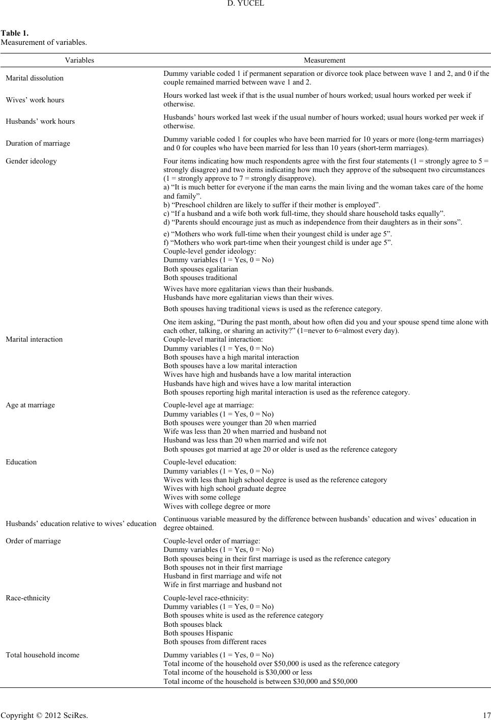

D. YUCEL
Table 1.
Measurement of variables.
Variables Measurement
Marital dissolution Dummy variable coded 1 if permanent separation or divorce took place between wave 1 and 2,and 0 if the
couple remained married between wave 1 and 2.
Wives’ work hours Hours worked last week if that is the usual number of hours worked; usual hours w orked per week if
otherwise.
Husbands’ wo r k hours Husbands’ hours worked last week if the usual numbe r of hours worked; usual hours worked per week if
otherwise.
Duration of marriage Dummy variable coded 1 for couples who have been married for 10 years or more (long-term marriages)
and 0 for couples who have been married for less than 10 years (short-term m arriages).
Gender ideology Four items indicating how much responde nts agree with the first four sta t ements (1 = s trongly agree to 5 =
strongly disagree) and two items indica ting how much they approve of t he subsequent two circumstances
(1 = strongly approve to 7 = strongly disapprove).
a) “It is much better for everyone i f the man earns th e main living and the woman takes care of the home
and family ”.
b) “Preschool children are likely to suffer if their mother is employed”.
c) “If a husband and a wi fe both work full-time, they should share household tasks equally”.
d) “Parents should encourage just as much as independence from their daughters as in their sons”.
e) “Mothers w ho work full-time when thei r youngest chil d is under age 5”.
f) “Mothers who work part-time when their youngest chil d is under age 5”.
Couple-level gender ide ology:
Dummy variables (1 = Yes, 0 = No)
Both spouses ega litarian
Both spouses traditional
Wives have more egalitarian views than their husbands.
Husbands have more egalitarian views tha n th eir wives.
Both spouses having traditional views is used as the reference category.
Marital interaction
One item asking, “During the past month, abo ut how often di d you and your spouse spend time alone with
each other, talking, or sharing an activity?” (1=never to 6=almost every day).
Couple-level marital interaction:
Dummy variables (1 = Yes, 0 = No)
Both spouses ha ve a high marital interaction
Both spouses ha ve a low marital in teraction
Wives have high and husban ds have a low marital interac tion
Husbands have high and wives have a low m arital interaction
Both spouses reporting high marita l interaction is us ed as the reference ca tegory.
Age at marriage Couple-leve l age at marriage:
Dummy variables (1 = Yes, 0 = No)
Both spouses were younger than 20 when married
Wife was less tha n 20 when married and husband not
Husband was less than 20 when married and w ife not
Both spouses got married at age 20 or older is used as the reference category
Education Couple-level education:
Dummy variables (1 = Yes, 0 = No)
Wives with less than high school degree is used as the reference category
Wives with high sc hool graduate degree
Wives with some college
Wives with college degree or more
Husbands’ educ ation relative to wives’ education Continuous va riable measured by the dif ference between husbands’ education and wives’ education in
degree obtained.
Order of ma rriage Couple-level order of m arriage:
Dummy variables (1 = Yes, 0 = No)
Both spouses being in their first marriage is used as the reference category
Both spouses not in their first marriage
Husband in first marriage and wife not
Wife in first marriage and hus band not
Race-ethnicity Couple-level race-ethnicity:
Dummy variables (1 = Yes, 0 = No)
Both spouses white is used as the reference category
Both spouses black
Both spouses Hispanic
Both spouses from different races
Total household income Dummy varia bles (1 = Yes, 0 = No)
Total income of the household o ver $50,000 is used as the reference category
Total income of the household is $30,000 or less
Total income of the household i s between $30,000 an d $50,000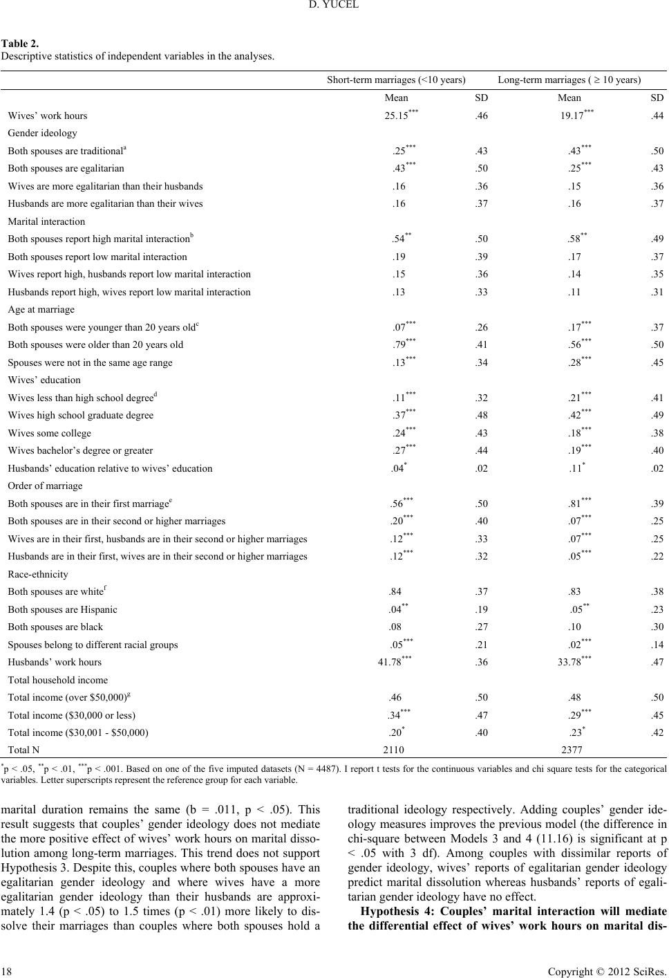

D. YUCEL
Table 2.
Descriptive statistics of independent variables in the analyses.
Short-term marriages (<10 years)Long-term marriages (10 years)
Mean SDMean SD
Wives’ work hours 25.15*** .46 19.17*** .44
Gender ideology
Both spouses are traditionala .25
*** .43 .43*** .50
Both spouses are e galitarian .43*** .50 .25*** .43
Wives are more egalitarian than their husbands .16 .36 .15 .36
Husbands are more egalitarian than their wives .16 .37 . 1 6 .37
Marital interaction
Both spouses report high marital interactionb .54
** .50 .58** .49
Both spouses re port low marita l i nt eraction .19 .39 . 17 .37
Wives report high, husbands report low marital interaction .15 .36 .14 .35
Husbands report high, wives re po rt low marital interaction .13 .33 .11 .31
Age at marriage
Both spouses were younger than 20 years oldc .07
*** .26 .17*** .37
Both spouses were older than 20 years old .79*** .41 .56*** .50
Spouses were not in the same age range .13*** .34 .28*** .45
Wives’ education
Wives less than high school degreed .11
*** .32 .21*** .41
Wives high school graduate degree .37*** .48 .42*** .49
Wives some c ollege .24*** .43 .18*** .38
Wives bachelor’s degree or greater .27*** .44 .19*** .40
Husbands’ education relative to wives’ education .04* .02 .11* .02
Order of marriage
Both spouses are in their first m arriagee .56
*** .50 .81*** .39
Both spouses are in their second or higher marriages .20*** .40 .07*** .25
Wives are in their first, husbands are in their second or higher marriages .12*** .33 .07*** .25
Husbands are in their first, wives are in their second or higher marriages .12*** .32 .05*** .22
Race-ethnicity
Both spouses are whitef .84 .37 .83 .38
Both spouses are Hispa nic .04** .19 .05** .23
Both spouses a re black .08 .27 .10 .30
Spouses belong to different racial groups .05*** .21 .02*** .14
Husbands’ work hours 41.78*** .36 33.78*** .47
Total household income
Total income (over $50,000)g .46 .50 .48 .50
Total income ($30,000 or less) .34*** .47 .29*** .45
Total income ($30,001 - $50,000) .20* .40 .23* .42
Total N 2110 2377
*p < .05, **p < .01, ***p < .001. Based on one of the five imputed datasets (N = 4487). I report t tests for the continuous variables and chi square tests for the categorical
variables. Letter superscripts represent the reference group for each variable.
marital duration remains the same (b = .011, p < .05). This
result suggests that couples’ gender ideology does not mediate
the more positive effect of wives’ work hours on marital disso-
lution among long-term marriages. This trend does not support
Hypothesis 3. Despite this, couples where both spouses have an
egalitarian gender ideology and where wives have a more
egalitarian gender ideology than their husbands are approxi-
mately 1.4 (p < .05) to 1.5 times (p < .01) more likely to dis-
solve their marriages than couples where both spouses hold a
traditional ideology respectively. Adding couples’ gender ide-
ology measures improves the previous model (the difference in
chi-square between Models 3 and 4 (11.16) is significant at p
< .05 with 3 df). Among couples with dissimilar reports of
gender ideology, wives’ reports of egalitarian gender ideology
predict marital dissolution whereas husbands’ reports of egali-
tarian gender ideology have no effect.
Hypothesis 4: Couples’ marital interaction will mediate
he differential effect of wives’ work hours on marital dis- t
1 8 Copyright © 2012 SciRes.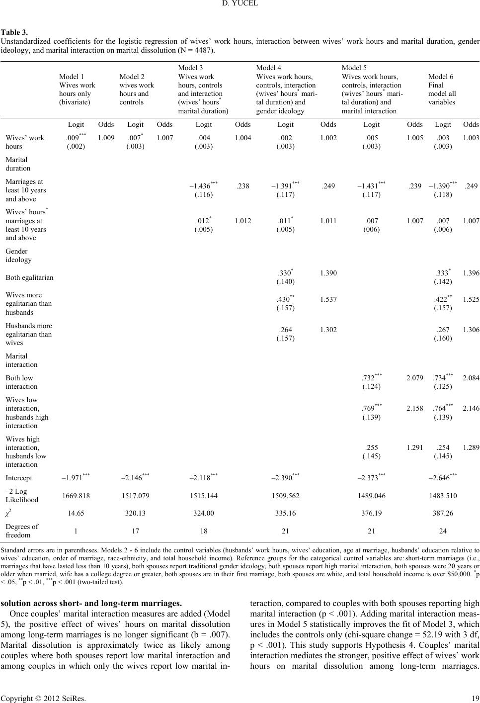

D. YUCEL
Table 3.
Unstandardized coefficients for the logistic regression of wives’ work hours, interaction between wives’ work hours and marital duration, gender
ideology, and marital interac tion on marital dissolution (N = 4487).
Model 1
Wives work
hours only
(bivariate)
Model 2
wives work
hours and
controls
Model 3
Wives work
hours, controls
and interaction
(wives’ hours*
marital duration)
Model 4
Wives work hour s,
controls, interaction
(wives’ hours* mari -
tal duration) and
gender ideolo gy
Model 5
Wives work hour s,
controls, interaction
(wives’ hours* mari -
tal duration) and
marital interaction
Model 6
Final
model all
variables
Logit Odds Logit Odds Logit OddsLogit OddsLogit Odds Logit Odds
Wives’ work
hours .009*** (.002) 1.009 .007* (.003) 1.007 .004 (.003) 1.004 .002 (.003) 1.002 .005 (.003) 1.005 .003 (.003) 1.003
Marital
duration
Marriages at
least 10 years
and above
–1.436***
(.116) .238 –1.391*** (.117) .249 –1.431*** (.117) .239 –1.390*** (.118) .249
Wives’ hours*
marriages at
least 10 years
and above
.012*
(.005) 1.012 .011* (.005) 1.011 .007 (006) 1.007 .007 (.006) 1.007
Gender
ideology
Both egalitarian .330*
(.140) 1.390
.333*
(.142) 1.396
Wives more
egalitarian than
husbands .430**
(.157) 1.537
.422**
(.157) 1.525
Husbands more
egalitarian than
wives .264
(.157) 1.302
.267
(.160) 1.306
Marital
interaction
Both low
interaction .732*** (.124) 2.079 .734*** (.125) 2.084
Wives low
interaction,
husbands high
interaction
.769***
(.139) 2.158 .764*** (.139) 2.146
Wives high
interaction,
husbands l o w
interaction
.255
(.145) 1.291 .254 (.145) 1.289
Intercept –1.971*** –2.146*** –2.118*** –2.390*** –2.373*** –2.646***
–2 Log
Likelihood 1669.818 1517.079 1515.144 1509.562 1489.046 1483.510
χ2 14.65 320.13 324.00 335.16 376.19 387.26
Degrees of
freedom 1 17 18 21 21 24
Standard errors are in parentheses. Models 2 - 6 include the control variables (husbands’ work hours, wives’ education, age at marriage, husbands’ education relative to
wives’ education, order of marriage, race-ethnicity, and total household income). Reference groups for the categorical control variables are: short-term marriages (i.e.,
marriages that have lasted less than 10 years), both spouses repo rt traditional gender id eology, both spous es report high marital inte raction, both sp ouses were 20 years or
older when married, wife has a college degree or greater, both spouses are in their first marriage, both spouses are white, and total household in come is over $50,00 0. *p
< .05, **p < .01, ***p < .001 (two- tailed test).
solution across short- and long-term marriages.
Once couples’ marital interaction measures are added (Model
5), the positive effect of wives’ hours on marital dissolution
among long-term marriages is no longer significant (b = .007).
Marital dissolution is approximately twice as likely among
couples where both spouses report low marital interaction and
among couples in which only the wives report low marital in-
teraction, compared to couples with both spouses reporting high
marital interaction (p < .001). Adding marital interaction meas-
ures in Model 5 statistically improves the fit of Model 3, which
includes the controls only (chi-square change = 52.19 with 3 df,
p < .001). This study supports Hypothesis 4. Couples’ marital
interaction mediates the stronger, positive effect of wives’ work
hours on marital dissolution among long-term marriages.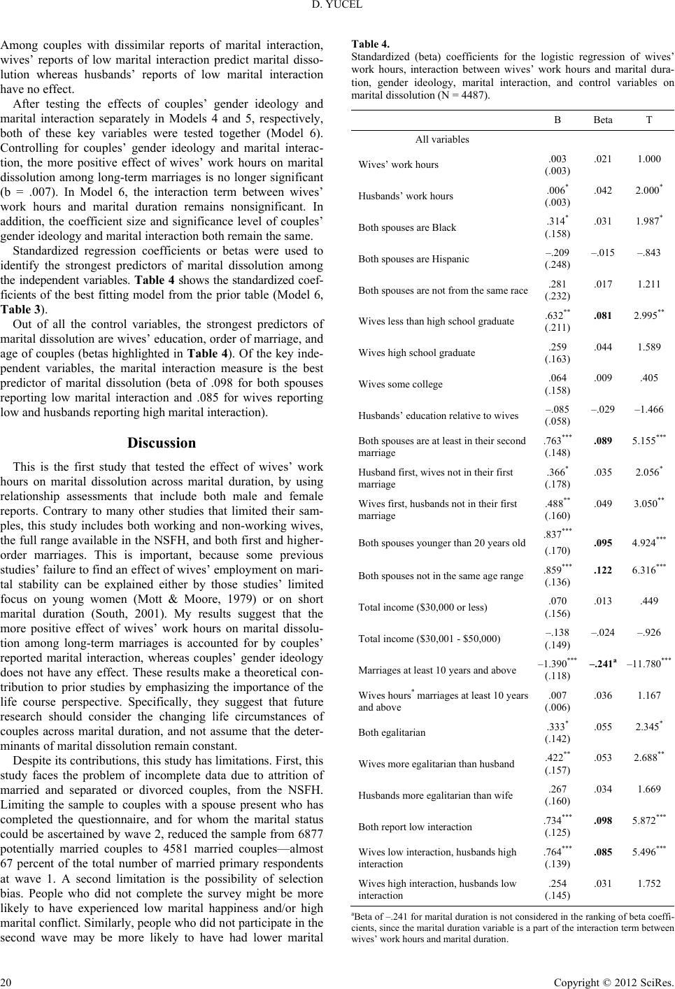

D. YUCEL
Among couples with dissimilar reports of marital interaction,
wives’ reports of low marital interaction predict marital disso-
lution whereas husbands’ reports of low marital interaction
have no effect.
After testing the effects of couples’ gender ideology and
marital interaction separately in Models 4 and 5, respectively,
both of these key variables were tested together (Model 6).
Controlling for couples’ gender ideology and marital interac-
tion, the more positive effect of wives’ work hours on marital
dissolution among long-term marriages is no longer significant
(b = .007). In Model 6, the interaction term between wives’
work hours and marital duration remains nonsignificant. In
addition, the coefficient size and significance level of couples’
gender ideology and marital interaction both remain the same.
Standardized regression coefficients or betas were used to
identify the strongest predictors of marital dissolution among
the independent variables. Table 4 shows the standardized coef-
ficients of the best fitting model from the prior table (Model 6,
Table 3).
Out of all the control variables, the strongest predictors of
marital dissolution are wives’ education, order of marriage, and
age of couples (betas highlighted in Table 4). Of the key inde-
pendent variables, the marital interaction measure is the best
predictor of marital dissolution (beta of .098 for both spouses
reporting low marital interaction and .085 for wives reporting
low and husbands reporting high marital interaction).
Discussion
This is the first study that tested the effect of wives’ work
hours on marital dissolution across marital duration, by using
relationship assessments that include both male and female
reports. Contrary to many other studies that limited their sam-
ples, this study includes both working and non-working wives,
the full range available in the NSFH, and both first and higher-
order marriages. This is important, because some previous
studies’ failure to find an effect of wives’ employment on mari-
tal stability can be explained either by those studies’ limited
focus on young women (Mott & Moore, 1979) or on short
marital duration (South, 2001). My results suggest that the
more positive effect of wives’ work hours on marital dissolu-
tion among long-term marriages is accounted for by couples’
reported marital interaction, whereas couples’ gender ideology
does not have any effect. These results make a theoretical con-
tribution to prior studies by emphasizing the importance of the
life course perspective. Specifically, they suggest that future
research should consider the changing life circumstances of
couples across marital duration, and not assume that the deter-
minants of marital dissolution remain constant.
Despite its contributions, this study has limitations. First, this
study faces the problem of incomplete data due to attrition of
married and separated or divorced couples, from the NSFH.
Limiting the sample to couples with a spouse present who has
completed the questionnaire, and for whom the marital status
could be ascertained by wave 2, reduced the sample from 6877
potentially married couples to 4581 married couples—almost
67 percent of the total number of married primary respondents
at wave 1. A second limitation is the possibility of selection
bias. People who did not complete the survey might be more
likely to have experienced low marital happiness and/or high
marital conflict. Similarly, people who did not participate in the
second wave may be more likely to have had lower marital
Table 4.
Standardized (beta) coefficients for the logistic regression of wives’
work hours, interaction between wives’ work hours and marital dura-
tion, gender ideology, marital interaction, and control variables on
marital dissolution (N = 4487).
B Beta T
All variables
Wives’ work hours .003
(.003) .021 1.000
Husbands’ wo r k hours .006*
(.003) .042 2.000*
Both spouses are Black .314*
(.158) .031 1.987*
Both spouses are Hispa nic –.209
(.248) –.015 –.843
Both spouses are not from the same race .281
(.232) .017 1.211
Wives less than high school graduate .632**
(.211) .081 2.995**
Wives high school graduate .259
(.163) .044 1.589
Wives some college .064
(.158) .009 .405
Husbands’ education relative to wives –.085
(.058) –.029 –1.466
Both spouses are at least in their second
marriage .763*** (.148) .089 5.155***
Husband first, wives not in their first
marriage .366* (.178) .035 2.056*
Wives first, husba nds not in their first
marriage .488** (.160) .049 3.050**
Both spouses younger than 20 years old .837***
(.170) .095 4.924***
Both spouses not in the same age range .859***
(.136) .122 6.316***
Total income ($30,000 or less) .070
(.156) .013 .449
Total income ($30,001 - $50,000) –.138
(.149) –.024 –.926
Marriages at least 10 yea rs and above –1.390***
(.118) –.241a –11.780***
Wives hours* marriages at least 10 years
and above .007 (.006) .036 1.167
Both egalitarian .333*
(.142) .055 2.345*
Wives more egalitarian than h usband .422**
(.157) .053 2.688**
Husbands more egalitarian than wife .267
(.160) .034 1.669
Both report low int eraction .734***
(.125) .098 5.872***
Wives low interaction, husbands high
interaction .764*** (.139) .085 5.496***
Wives high inte raction, husbands low
interaction .254 (.145) .031 1.752
aBeta of –.241 for marital duratio n is not considered in th e ranking of beta co effi-
cients, since the marit al duration variable is a part of th e interaction term between
wives’ work hours and marital duration.
2 0 Copyright © 2012 SciRes.

D. YUCEL
quality and to have divorced. Overall, some previous studies
concluded that several factors measured in wave 1 of the NSFH
significantly predict attrition by wave 2 (Mirowsky & Reynolds,
2000; Simon, 2002). These studies showed that the results dif-
fer significantly, depending on whether they ignore attrition or
adjust the models to compensate for the hazard of attrition.
Lastly, I would need more than two waves of data to rule out
the causal role of wives’ work hours on marital dissolution.
Thus, the results presented in this study should be classified as
“correlates” and not true “causes” of marital dissolution.
This study also suggests some possible avenues for future
research. One would be to use the third wave of NSFH data.
The same question could be explored by studying married cou-
ples at wave 1 and looking at their outcomes in wave 3, which
was conducted from 2001 to 2002. Using all three waves would
provide researchers with a dataset spanning fifteen years, and
enable them to include changes in employment and marital
interaction as well as changes in gender ideology between the
first two waves. It would also allow them to analyze the effects
of these changes on the marital outcome in wave 3. One could
also compare couples married at wave 2 with wave 2 employ-
ment patterns, to predict dissolution by wave 3. These analyses
would permit examination of whether the adverse effects of
wives’ work hours may have decreased in recent years (i.e., to
test whether the effect of wives’ work hours on marital dissolu-
tion varies depending on the year of observation, consistent
with the findings of South (2001)). Despite the advantages of
using all three waves of data, a serious problem would result
from the attrition rate. Due to funding constraints, wave 3 does
not include any respondents under age 45 as of January 2000
(or their spouses) who did not have a wave 1 focal child eligible
to be interviewed at wave 2 (Sweet & Bumpass, 2002).
Overall, the results conclude that socioeconomic indicators
such as wives’ employment may have differential effects on
marital dissolution across marital duration. This more positive
relationship between marital quality and stability among long-
term marriages (where there is external pressure to remain mar-
ried due to the existence of greater barriers and fewer alterna-
tives) is consistent with Lewis and Spanier’s social exchange
theory (1979). The results are also consistent with Schmitt et al.
(2007), who also suggest that more research and theoretical
development are required to understand better the determinants
of marital dissolution across marital duration. Using couple-
level data such as those provided by the NSFH (which collects
information from both spouses and measurement approaches) is
critical to further progress in this area. Moreover, this study
advances the testing of some of the key indicators that explain
the differential effect of wives’ work hours on marital dissolu-
tion across short- and long-term marriages. Future studies
should test other indicators that might mediate or moderate the
varying effects of wives’ work hours on marital dissolution
across marital duration, such as the quality of marital interac-
tion (how spouses interact with one another), depression, health
status, or social networks.
Acknowledgements
I appreciate the comments of Dr. Douglas Downey, Dr.
Margaret Gassanov, and Dr. Donna Bobbitt-Zeher.
REFERENCES
Allison, P. D. (2002). Missing data. Thousand Oak s, CA: Sage.
Austen, S. (2004). Labour supply and the risk of divorce: An analysis
of Australian data. Australian Economic Review, 37, 153-165.
doi:10.1111/j.1467-8462.2004.00316.x
Booth, A., & Edwards, J. N. (1985). Age at marriage and marital insta-
bility. Journal of Marriage and Family, 47, 67-75.
doi:10.2307/352069
Booth, A., Johnson D. R., White, L. K., & Edwards, J. N. (1984).
Women, outside employment, and marital instability. American
Journal of Sociology, 90, 567-583. doi:10.1086/228117
Booth, A., Johnson, D. R., White, L. K., & Edwards, J. N. (1985).
Predicting divorce and permanent separation. Journal of Family Is-
sues, 6, 331-346. doi:10.1177/019251385006003005
Booth, A., Johnson, D. R., White, L. K., & Edwards, J. N. (1986).
Divorce and marital instability over the life course. Journal of Fam-
ily Issues, 7, 421-442. doi:10.1177/019251386007004006
Bumpass, L. L. (1990). What’s happening to the family? Interactions
between demographic and institutional change. Demography, 27,
483-498. doi:10.2307/2061566
Bumpass, L. L., Martin, T. C., & Sweet, J. A. (1991). The impact of
family background and early marital factors on marital disruption.
Journal of Family Issues, 12, 22-42.
doi:10.1177/019251391012001003
Cunningham, M. (2001). The influence of parental attitudes and be-
haviors on children’s attitudestoward gender and household labor in
early adulthood. Journal of Marriage and Family, 63, 111-122.
doi:10.1111/j.1741-3737.2001.00111.x
Esterberg, K. G., Moen, P., & Dempster-McClain, D. (1994). Transi-
tion to divorce: A life-course approach to women’s marital duration
and dissolution. The Sociological Quarterly, 35, 289-307.
doi:10.1111/j.1533-8525.1994.tb00411.x
Frisco, M. L., & Williams, K. (2003). Perceived housework equity,
marital happiness, and divorce in dual-earner households. Journal of
Family Issues, 24, 51-73. doi:10.1177/0192513X02238520
Gager, C. T., & Sanchez, L. (2003). Two as one? Couples’ perceptions
of time spent together, marital quality, and the risk of divorce. Jour-
nal of Family Issues, 24, 21-50. doi:10.1177/0192513X02238519
Gershuny, J., Bittman, M., & Brice, J. (2005). Exit, voice, and suffering:
Do couples adapt to changing employment patterns? Journal of Mar-
riage and Family, 67, 656 -665.
doi:10.1111/j.1741-3737.2005.00160.x
Gray, J. S. (1995). The causality between employment and divorce.
Family Economics and Resources Management Biennial, 1, 171-176.
Greene, W. H., & Quester, A. Q. (1982). Divorce risk and wives’ labor
supply behavior. Social Science Quarterly, 63, 16-27.
Greenstein, T. N. (1990). Marital disruption and the employment of
married women. Journal of Marriage and Family, 52, 657-676.
doi:10.2307/352932
Greenstein, T. N. (1995). Gender ideology, marital disruption, and the
employment of married women. Journal of Marriage and Family, 57,
31-42. doi:10.2307/353814
Greenstein, T. N. (1996). Gender ideology and perceptions of the fair-
ness of the division of household labor: Effects on marital quality.
Social Forces, 74, 1029- 1042.
Hatch, L. R., & Bulcroft, K. (2004). Does long-term marriage bring less
frequent disagreements? Five explanatory frameworks. Journal of
Family Issues, 25, 465-495. doi:10.1177/0192513X03257766
Heaton, T. B. (1991). Time-related determinants of marital dissolution.
Journal of Marriage and Family, 53, 285-295.
doi:10.2307/352899
Heaton, T. B., Albrecht, S. L., & Martin, T. K. (1985). The timing of
divorce. Journal of Marriage and Family, 47, 631-640.
doi:10.2307/352264
Hill, M. S. (1988). Marital stability and spouses’ shared time. Journal
of Family Issues, 9, 427-451. doi:10.1177/019251388009004001
Hochschild, A. R., & Machung, A. (1989). The second shift. New York,
NY: Avon.
Johnson, J. H. (2004). Do long work hours contribute to divorce? Top-
ics in Economic Analysis and Policy, 4, 1-23.
doi:10.2202/1538-0653.1118
Johnson, W. R., & Skinner, J. (1986). Labor supply and marital separa-
tion. American Economic Review, 76, 455-469.

D. YUCEL
22 Copyright © 2012 SciRes.
Karney, B. R., & Bradbury, T. N. (1995). The longitudinal course of
marital quality and stability: A review of theory, method, and re-
search. Psychological Bulletin, 118, 3-34.
doi:10.1037/0033-2909.118.1.3
Kenrick, D. T., Linsenmeier, J. A. W., Norman, P. L., & Bailey, J. M.
(2002). The necessities and luxuries of mate preferences: Testing the
tradeoffs. Journal of Personality and Social Psychology, 82, 947-
955. doi:10.1037/0022-3514.82.6.947
Kingston, P. W., & Nock, S. L. (1987). Time together among dual-
earner couples. American Sociological Review, 52, 391-400.
doi:10.2307/2095358
Levinger, G. (1979). A social psychological perspective on marital
dissolution. In G. Levinger, & O. C. Moles (Eds.), Divorce and
separation (pp. 36- 70). New York, NY: Basic.
Lewis, R. A., & Spanier, G. B. (1979). Theorizing about the quality and
stability of marriage. In W. Burr, R. Hill, F. I. Nye, & I. Reiss (Eds.),
Contemporary theories about the family (pp. 268-294). New York,
NY: Free Press.
Lye, D. N., & Biblarz, T. J. (1993). The effects of attitudes toward
family life and gender roles on marital satisfaction. Journal of Fam-
ily Issues, 14, 157-188. doi:10.1177/019251393014002002
Mirowsky, J., & Reynolds, J. R. (2000). Age, depression, and attrition
in the national survey of families and households. Sociological
Methods and Research, 28, 476-504.
doi:10.1177/0049124100028004004
Montalto, C. P., & Gerner, J. L. (1998). The effect of expected changes
in marital status on labor supply decisions of women and men. Jour-
nal of Divorce and Remarriage, 28, 25-51.
doi:10.1300/J087v28n03_02
Morgan, S. P., & Rindfuss, R. R. (1985). Marital disruption: Structural
and temporal dimensions. American Journal of Sociology, 90, 1055-
1077. doi:10.1086/228176
Mott, F. L., & Moore, S. F. (1979). The causes of marital disruption
among young American women: An interdisciplinary perspective.
Journal of Marriage and Family, 41, 355-365. doi:10.2307/351702
Papps, K. L. (2006). The effects of divorce risk on the labor supply of
married couples. IZA Discussion Paper, No. 2395.
Poortman, A. (2005). How work affects divorce: The mediating role of
financial and time pressures. Journal of Family Issues, 26, 168-195.
doi:10.1177/0192513X04270228
Presser, H. B. (2000). Nonstandard work schedules and marital insta-
bility. Journal of Marriage and Family, 62, 93-110.
doi:10.1111/j.1741-3737.2000.00093.x
Rogers, S. J. (1999). Wives’ income and marital quality: Are there
reciprocal effects? Journal of Marriage and Family, 61, 123-132.
doi:10.2307/353888
Sanchez, L., & Gager, C. T. (2000). Hard living, perceived entitlement
to a great marriage, and marital dissolution. Journal of Marriage and
Family, 62, 708-722. doi:10.1111/j.1741-3737.2000.00708.x
Sayer, L. C., & Bianchi, S. M. (2000). Women’s economic independ-
ence and the probability of divorce: A review and reexamination.
Journal of Family Issues, 21, 906-943.
doi:10.1177/019251300021007005
Schmitt, M., Kliegel, M., & Shapiro, A. (2007). Marital interaction in
middle and old age: A predictor of marital satisfaction? The Interna-
tional Journal of Aging and Human Development, 65, 283-300.
doi:10.2190/AG.65.4.a
Schoen, R. (1975). California divorce rates by age at first marriage and
duration of first marriage. Journal of Marriage and the Family, 37,
548-555. doi:10.2307/350518
Schoen, R., Astone, N. M., Rothert, K., Standish, N. J., & Kim, Y. J.
(2002). Women’s employment, marital happiness, and divorce. So-
cial Forces, 81, 643-662. doi:10.1353/sof.2003.0019
Schoen, R., Rogers, S. J., & Amato, P. R. (2006). Wives’ employment
and spouses’ marital happiness: Assessing the direction of influence
using longitudinal couple data. Journal of Family Issues, 27, 506-528.
doi:10.1177/0192513X05283983
Schoen, R., & Wooldredge, J. (1989). Marriage choices in North Caro-
lina and Virginia, 1969-1971 and 1979-1981. Journal of Marriage
and the Family, 51, 46 5-481. doi:10.2307/352508
Sen, B. (2000). How important is anticipation of divorce in married
women’s labor supply decisions? An intercohort comparison using
NLS data. Economics Letters, 67, 209-216.
doi:10.1016/S0165-1765(99)00259-1
Simon, R. W. (2002). Revisiting the relationships among gender, mari-
tal status, and mental health. American Journal of Sociology, 107,
1065-1096. doi:10.1086/339225
Smith-Lovin, L., & Tickamyer, A. R. (1978). Nonrecursive models of
labor force participation, fertility behavior, and sex role attitudes.
American Sociological Review, 43, 541- 55 7. doi:10.2307/2094778
South, S. J. (2001). Time-dependent effects of wives’ employment on
marital dissolution. American Sociological Review, 66, 226-245 .
doi:10.2307/2657416
South, S. J., & Spitze, G. (1986). Determinants of divorce over the
marital life course. American Sociological Review, 51, 583-590.
doi:10.2307/2095590
Spitze, G., & South, S. J. (1985). Women’s employment, time expen-
diture, and divorce. Journal of Family Issues, 6, 307-329.
doi:10.1177/019251385006003004
Sweet, J. A., & Bumpass, L. L. (1987). American families and house-
holds. New York: Russell Sage Foundation.
Sweet, J. A., & Bumpass, L. L. (2002). The national survey of families
and households—Waves 1, 2, and 3: Data description and documen-
tation. Madison: Center for Demography and Ecology, University of
Wisconsin-Madison.
Sweet, J. A., Bumpass, L. L., & Call, V. A. (1988). The design and
content of the national survey of families and households. Madison:
Center for Demography and Ecology, University of Wisconsin-
Madison.
Voydanoff, P. (1988). Work role characteristics, family structure de-
mands, and work/family conflict. Journal of Marriage and Family,
50, 749-761. doi:10.2307/352644
Wentworth, D. K., & Chell, R. M. (2005). Gender identity at home:
Comparing the role of househusband to housewife. In J. W. Lee ( Ed.),
Psychology of gender identity (pp. 113-126). Hauppauge, NY: Nova
Biomedical.
White, L. K., & Booth, A. (1991). Divorce over the life course: The
role of marital happiness. Journal of Family Issues, 12, 5-21.
doi:10.1177/019251391012001002
Wilkerson, J. A., Yamawaki, N., & Downs, S. D. (2009). Effects of
husbands’ migration on mental health and gender role ideology of
rural Mexican women. Health Care for Women International, 30,
612-626. doi:10.1080/07399330902928824