Open Journal of Statistics, 2012, 2, 48-59
http://dx.doi.org/10.4236/ojs.2012.21006 Published Online January 2012 (http://www.SciRP.org/journal/ojs)
Minimum MSE Weights of Adjusted Summary
Estimator of Risk Difference in Multi-Center Studies
Chukiat Viwatwongkasem1*, Jirawan Jitthavech2, Dankmar Böhning3, Vichit Lorchirachoonkul2
1Department of Biostatistics, Faculty of Public Health, Mahidol University, Bangkok, Thailand
2School of Applied Statistics, National Institute of Development Administration, Bangkok, Thailand
3Applied Statistics, School of Biological Sciences, University of Reading, Reading, UK
Received October 14, 2011; revised November 18, 2011; accepted November 30, 2011
ABSTRACT
The simple adjusted estimator of risk difference in each center is easy constructed by adding a value c on the number of
successes and on the number of failures in each arm of the proportion estimator. Assessing a treatment effect in
multi-center studies, we propose minimum MSE (mean square error) weights of an adjusted summary estimate of risk
difference under the assumption of a constant of common risk difference over all centers. To evaluate the performance
of the proposed weights, we compare not only in terms of estimation based on bias, variance, and MSE with two other
conventional weights, such as the Cochran-Mantel-Haenszel weights and the inverse variance (weighted least square)
weights, but also we compare the potential tests based on the type I error probability and th e power of test in a variety
of situations. The results illustrate that the propo sed weights in terms of point estimation and hypothesis testing perform
well and should be recommend ed to use as an alternative choice. Finally, two ap plications are illustrated for the practi-
cal use.
Keywords: Minimum MSE Weights; Optimal Weights; Cochran-Mantel-Haenszel Weights; Inverse Variance Weights;
Multi-Center Studies; Risk Difference
1. Introduction
It is widely known that the conventional proportion esti-
mator, ˆ
pXn, is a maximum likelihood estimator
(MLE) and an uniformly minimum variance unbiased
estimator (UMVUE) for the binomial parameter p
where the binomial random variable
X
is the number
of successes out of the number of patients n. However,
Agresti and Coull [1], Agresti and Caffo [2], Ghosh [3],
and Newcombe [4,5] highlighted the point that ˆ
p might
not be a good choice for p when the assumption of
ˆ5np  and

ˆ 15np was violated; this violation
often occurs when the sample size n is small, or the
estimated probability ˆ
p is close to 0 or 1 (close to the
boundaries of parameter space), leading to the problem
of the zero estimate of the variance of ˆ
p. The estimated
variance of ˆ
p, provided by


ˆˆ ˆ
() 1Vppp n , is zero
in the occurrence of any case: 0X or
X
n

. Böh-
ning and Viwatwongkasem [6] proposed the simple ad-
justed proportion estimator by adding a value c on the
number of successes and the number of failures; cones-
quently,
 
ˆ2
c
pXcnc is their proposed esti-
mate of p with the non-zero variance estimate

  
2
ˆˆˆ
12
ccc
Vpnppn c . They concluded that the
estimator




12Xn

 minimizes the Bayes risk (the
average MSE of ˆc
p) in the class of all estimators of the
form




2
X
cnc with respect to uniform prior on
[0,1] and Euclidean loss function; furthermore, the esti-
mator




12Xn

 has smaller MSE than
X
n in
the approximate interval


0.15,0.85 of p. For another
argumentation in the Bayesian approach, Casella and
Berger [7] showed that

 
Xn

 
is a Bayes
estimator of p under the conditional b inomial sampling


~,
X
pbinomialn p and the prior beta distribution


~,pbeta

 . Note that in case of 1

  the beta
distribution has a special case as the uniform distribution
over [0,1]. Consequently, the estimator



2
X
cnc
derived from the Bayesian approach and the Bayes risk
approach und er the ab ove men tion ed crite ria pr ovid es th e
same result at 1c

.
With the idea of

 
ˆ2
c
pXcnc , the extension
leads to 12
ˆˆˆ
ccc
pp  , the adjusted risk difference esti-
mator between two independent binomial proportions,
for estimating a common risk difference

where




11111
ˆ2
c
pXcnc and



22222
ˆ2
c
pXcnc 
are proportion estimators for treatment and control arms.
In a multi-center study of size k, the parameter of in-
*Corresponding author.

C. VIWATWONGKASEM ET AL.
49
terest is also a common risk difference

that is as-
sumed to be a constant across centers. We concern about
a combination of several adjusted risk difference estima-
tors 12
ˆˆˆ
cjc jcj
pp

 from the th j center


1, 2,,jk
into the adjusted summary estimator of risk difference of
the form 1
ˆˆ
k
cwcj cj
jf



 where cj
f
are the weights
subject to the condition that 11
k
cj
jf 
. In this study,
we would propose the optimal weights cj
f
as an alter-
native choice based on minimizing the MSE of ˆcw

in
Section 2, then state the well-known candidates such as
the Cochran-Mantel-Haenszel (CMH) weights and the
inverse variance (INV) weights in Section 3. A simula-
tion plan for comparing the performance among weights
in terms of estimation and hypothesis testing is presented
in Section 4. The results of the comparison among the
potential estimators based on bias, variance, and MSE
and also the evaluations among tests related the men-
tioned weights through the type I error probability and
the power criteria lie on Section 5. Some numerical ex-
amples are applied in Section 6. Finally, conclusion and
discussion are presented in Section 7.
2. Deriving Minimum MSE Weights of
Adjusted Summary Estimator
Under the assumption of a constant of common risk dif-
ference

across k centers, we combine several ad-
justed risk difference estimators 12
ˆˆˆ
cjc jcj
pp   in
which
 
11111
ˆ2
cj jj
pXcnc  and
 
22222
ˆ2
cj jj
pXcnc  from the th j center

1, 2,,jk arrive at an adjusted summary estimator
of risk difference of the form 1
ˆˆ
k
cwcj cj
jf



 where
cj
f
are non-random weights subject to the constraint
that 11
k
cj
jf 
. Please observe that for a single center

1k the adju sted summary estimator 1
ˆˆ
k
cwcj cj
jf




subject to 11
k
cj
jf 
 is a shrinkage estimator of a
simple adjusted estimator 12
ˆˆˆ
ccc
pp  . Our minimum
MSE weights cj
f
of the adjusted summary estimator
ˆcw

were derived by following Lagrange’s method [8]
under the assumption of a constant of common risk dif-
ference over all centers with the pooling point estimator
to estimate

. Lui and Chang [9] proposed the optimal
weights proportional to the reciprocal of the variance
with the Mantel-Haenszel point estimator under the as-
sumption of noncompliance. It was observ ed that both of
optimal weights provided the different formulae because
of different assumptions even though they were derived
from the same method of Lagrange. Now, we wish to
present the proposed weights minimizing the MSE of
ˆcw

as follows:
 
2
2
1
ˆˆ ˆ
k
cwcwcjc j
j
QMSEEE f

 


 



To obtain the minimum Q subject to a constraint
11
k
jcj
f



, we form the auxiliary function

to seek
cj
f
that minimize
2
11
ˆ1
kk
cj cjcj
jj
Ef f 



 



where

is a Lagrange multiplier. The weights cj f
and

are derived by solving the following equations
simultaneously: 0




, 0
cj
f


, 1,2,,jk. The
details are presented in Appendix. The result of the
weighted estimate for the th j center yields



1
1
11
1
1
ˆ ˆˆ
1
ˆˆ
ˆ
ˆˆ
ˆˆ
1
ˆ
ˆˆˆ
ˆˆ
jj pool
cj
k
mmmm pool
jj
k
mmmm
V
fa
VE
V
a
aEV


























where 1112 22
112 2
ˆˆ
ˆ22
jcj jcj
jjj
npc npc
Enc nc









111222
22
112 2
ˆˆˆˆ 11
ˆ22
j
cj cjjcj cj
j
jj
npp npp
Vnc nc



, ˆ
ˆ
ˆˆ
jj
aE b 


1
11
1ˆ
ˆˆ
kk
j
jj
j
aV
V




, 1
ˆ
ˆˆ
k
j
j
j
E
bV



, 12
ˆˆˆ
pool pp
 
11 1
11
1
11
11
ˆ
ˆ
kk
j
jj
jj
kk
j
j
jj
np X
pnn





,
22 2
11
2
22
11
ˆ
ˆ
kk
j
jj
jj
kk
j
j
jj
np X
pnn





In the particular case of 12 0cc, our estimator
1
ˆˆ
k
cwjcjcj
f





has a shrinkage estimator to be the
popular inverse-variance weighted estimator. Under a
common risk difference

over all centers, the variance
of ˆcw

in the case of non-random weights cj
f
are ob-
tained by
 




2
1
1112 22
222
1112 2
ˆˆ
11
22
k
cwcjcj
j
kjjjj jj
cj
jjj
VfV
npp npp
fncnc













Suppose that a normal approximation is reliable, the
asymptotic distribution is
 
1
2
1
ˆˆ
ˆ(0,1)
ˆ ˆˆ ˆˆ
k
cj cj
j
cw
k
cwcj cj
j
fN
VfV










C. VIWATWONGKASEM ET AL.
50
for testing 00
:H

  we have the norm al approximate test

0
1
20
1
ˆˆ
ˆˆ ˆ
k
cj cj
j
cw k
cjcj
j
f
Z
f
VH







We will reject 0
H
at

level for two-sided test if
2cw
Z
Z

 where 2
Z

is the upper


100 2th 
percentile of the standard normal distribution. Alterna-
tively, 0
H
is rejected when the p-value (p) is less than
or equal to


p

 where


21 cw pZ



and


Z
 is the standard cumulative normal distribu-
tion function.
3. Other Well-Known Weights
3.1. Cochran-Mantel-Haenszel (CMH) Weights
Cochran [10,11] proposed a weighted estimator of cen-
ter-specific sample sizes for a common risk difference
based on the unconditional binomial likelihood as
1
1
ˆ
ˆk
j
j
j
CMH
j
k
j
w
w






where

1
121 2
12
11
j
jj jj
jj
wnnnn
nn


 


 and
12
12 12
ˆˆˆ
j
j
jjj
j
j
X
X
pp nn
  . Cochran’s weight
j
w is
widely used as a standard non-random weight derived by
the harmonic means of the center-specific sample sizes.
Note that 1
k
j
jj
j
fw w

 is also Cochran’s weight
subject to the condition that 11
k
j
jf 
. A straightfor-
ward derivation illustrates that ˆCMH  is an unbiased
estimate of

and the variance of ˆCMH  is readily
available as
 

2
1
2
1
ˆ
ˆ
k
j
j
j
CMH k
j
j
wV
Vw






where

 
1112 22
ˆ11
j
jjjjjj
Vppnppn   . As-
suming that a normal approximation is reliable, the
Cochran’s Z-statistic for testing 00 :H

  is provided
as

  
0
2
20
11
11
ˆ
ˆ ˆ
jj j
CMH
jj j
kk
jj
kk
jj
ww
Z
wV Hw







where

 
01 11222
ˆ ˆˆˆˆˆ
11
j
jjjjjj
VHp pnppn   .
The rejection rule of 0
H
follows the same as the previ-
ous standard normal test.
Alternatively, Mantel and Haenszel [12] suggested the
test based on the conditional hypergeometric likelihood
for a common odds ratio among the set of k tables un-
der the null hypothesis of 0:1HOR

0 

. With
the null criterion, Mantel-Haenszel’s weight stated by
Sanchez-Meca and Marin-Martine [13] was equivalent to


1212 1 jjjjj
wnn nn

. Since the minor difference
between the conditional Mantel-Haenszel weight and the
unconditional Cochran weight is in the denominators,
thus the two are often referred to interchangeably as the
Cochran-Mantel-Haenszel weight. In this study, we use


121 2
j
jj j j
wnnnn.
3.2. Inverse Variance (INV) or Weighted Least
Square (WLS) Weights
Fleiss [14] and Lipsitz et al. [15] showed that the in-
verse-variance weighted (INV) estimator or the weighted-
least-square (WLS) estimator for

was in the summa ry
estimator of the weighted mean (linear, unbiased estima-
tor) of th e form
11
ˆˆ
kk
I
NVj jj
jj
ww 




where 1211 22
ˆˆˆ
j
jj jj jj
pp XnXn    and
j
w de-
fined by the reciprocal of the variance as


1
1122
12
11
1ˆ
jjj j
jjj
j
pppp
wnn
V 




 


The non-random and non-negative weights
j
w yield
the minimum variance of the summary estimator ˆ
I
NV

for estimating

. The variance of ˆ
I
NV
 is just given by




22
22
11
1
11
ˆ11
ˆjj jj
INV
j
jj
kk
jj
k
kk
j
jj
wV ww
Vw
ww







 



However, the weights
j
w cannot be used in practice
since 1
j
p and 2
j
p are unknown. Therefore, it has be-
come common practice to replace them by their sample
estimators. It yields


1122
1
12
ˆˆ ˆˆ
11
ˆ
j
jj j
jjj
pppp
wnn


This weight was suggested in several textbooks of
epidemiology such as Kleinbaum et al. [16] or in text-
books of meta-analysis such as Petitt [17]. We assume
that a normal approximation is reliable; the inverse-variance
weighted test statistic for testing 00 :H

  is






0
11
1
ˆ
1
jj
j
INV
j
kk
jj
k
j
ww
Zw







where


10
ˆ ˆ
ˆjj
wV H 
. Also, the rule of 0
H
rejection
follows the same as the above standard normal test.

C. VIWATWONGKASEM ET AL.
51
4. Monte Carlo Simulation
We perform simulations for estimating a common risk
difference

and testing the null hypothesis 00 :H



in the similar plans as follows:
Parameters Setting: Let the common risk difference

be some constants varying from 0 to 0.6, with incre-
mental steps of 0.1. Baseline proportion risks 2
j
p

21 222
,,,
k
pp p in the control arm for the th j center


1, 2,,jk are generated from a uniform distribution
over


0, 0.95

. The correspondent proportion risks
1
j
p for the treatment arm in the th j cen ter ar e ob ta in ed
as 12jj pp

. For example, if 0.2

, then

2~0,0.75 j
pU and

12 ~ 0.2,0.95 jj
pp U   . The
sample sizes 1
j
n and 2
j
n are varied as 4, 8, 16, 32,
100. The number of centers k takes values 1, 2, 4, 8, 16,
32.
Statistics: Binomial random variables 1
j
X
and 2
j
X
in treatment and control arms are generated with pa-
rameters

11
,
j
j
np and

22
,
j
j
np for each center j.
Estimation: All summary estimates of

are com-
puted in a variety of different weights. The procedure is
replicated 5000 times. From these replicates, bias, vari-
ance, and MSE (mean square error) are computed in the
conventional way.
Type I Error: From the above parameter setting, we
assign 0

  under a null 00 :H

 , so all tests are
computed. The replication is treated 5000 times. From
these replicates, the number of the null hypothesis reject-
tions is counted for the empirical type I error


.

00
Number of rejections of when is true
Number of replications (5000 times)
HH
 
The evaluation for two-sided tests in terms of the type
I probability is based on Cochran limits [18] as follow.
At 0.01

, the


value is between


0.005, 0.015.
At 0.05

, the


value is between


0.04, 0.06.
At 0.10

, the


value is between


0.08, 0.12.
If the empirical type I error ˆ

lies within those of
Cochran limits, then the statistical test can control type I
error.
Power of Tests: Before evaluating tests with their
powers, all comparative tests should be calibrated to have
the same type I error rate under 0
H
; then any test whos e
power hits the maximum under 1
H
would be the best
test. To achieve the alternative hypothesis, we assume
the random effect model for
j

as

0.10.12 1
jm
UmU  
where m U as an effect of between centers is assigned to
be uniform


,mm for a given


0, 0.1m, or
equivalently, U is an uniform variable over


0,1.
That is,

0.1
j
E   and


2
212
j
Var m  . Also,
we have 12
j
jj
pp

 where 2
j
p be uniform distri-
bution over


0.1, 0.8. Binomial random variables 1
j
X
and 2
j
X
are drawn with parameters

11
,
j
j
np, and


22
,
j
j
np, respectively. All proposed test statistics are
then computed. The procedure is replicated 5,000 times.
From these replicates, the empirical power

1


of test
is counted.


01
Number of rejections of when is true
1
Number of replications 5000 times
H
H
 
5. Results
Since it is difficult to present all enormous results from
the simulation study, we just have illustrated some in-
stances. Nevertheless, the main results are concluded
perfectly.
5.1. Results for Estimating Risk Differences
Table 1 presents some results according to point estima-
tion of a common risk difference

. However, we can
draw conclusions in the following.
 The number of centers, k, can not change the order
of the MSE of all weighted estimators, even though
an increase in k can decrease the variance and the
MSE of all estimators, leading to the increasing effi-
ciency. Also, increasing 1
j
n and 2
j
n can decrease
the variance of all estimators while fixing k. The
unbalanced cases of 1
j
n and 2
j
n for center j have
a rare effect on the order of the MSE of all estim ates.
 For most popular situations used under 0


,
0.1


, 0.2


, and 0.3

, the proposed sum-
mary estimator

cw

adjusted by 12 1ccc in-
cluding adjusted by 2c

is the best choice with the
smallest MSE. The estimator ˆcw

adjusted by
0.5c

and the inverse-variance (INV) weighted es-
timator


0c

are close tog ether and ar e the second
choice with smaller MSE. The Cochran-Mantel-
Haenszel (CMH) weight performs the worst in this
simulation setting. This finding is very useful in gen-
eral situations of most clinical trials and most causal
relations between a disease and a suspected risk factor
since the risk difference is often less than 0.25 [19].
 For 0.4


, the proposed estimator ˆcw

adjusted
by 1c

performs best; for 0.5

, the proposed
estimator ˆcw

adjusted by 0.5c performs best;
for 0.6


, the INV weighted estimator (0c

)
performs best.
5.2. Results for Studying Type I Error
Table 2 presents some results for controlling the empiri-
cal type I error. We can conclude the performance of
several tests according to the empirical alpha under 0
H
as follows.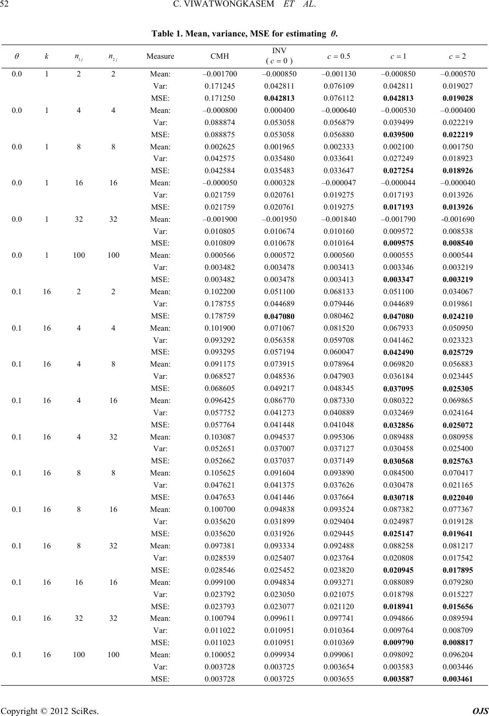

C. VIWATWONGKASEM ET AL.
52
Table 1. Mean , variance, M SE for estimating θ.

k 1j
n 2j n Measure CMH INV
(0c

) 0.5c 1c 2c

0.0 1 2 2 Mean: –0.001700 –0.000850 –0.001130 –0.000850 –0.000570
Var: 0.171245 0.042811 0.076109 0.042811 0.019027
MSE: 0.171250 0.042813 0.076112 0.042813 0.019028
0.0 1 4 4 Mean: –0.000800 0.000400 –0.000640 –0.000530 –0.000400
Var: 0.088874 0.053058 0.056879 0.039499 0.022219
MSE: 0.088875 0.053058 0.056880 0.039500 0.022219
0.0 1 8 8 Mean: 0.002625 0.001965 0.002333 0.002100 0.001750
Var: 0.042575 0.035480 0.033641 0.027249 0.018923
MSE: 0.042584 0.035483 0.033647 0.027254 0.018926
0.0 1 16 16 Mean: –0.000050 0.000328 –0.000047 –0.000044 –0.000040
Var: 0.021759 0.020761 0.019275 0.017193 0.013926
MSE: 0.021759 0.020761 0.019275 0.017193 0.013926
0.0 1 32 32 Mean: –0.001900 –0.001950 –0.001840 –0.001790 -0.001690
Var: 0.010805 0.010674 0.010160 0.009572 0.008538
MSE: 0.010809 0.010678 0.010164 0.009575 0.008540
0.0 1 100 100 Mean: 0.000566 0.000572 0.000560 0.000555 0.000544
Var: 0.003482 0.003478 0.003413 0.003346 0.003219
MSE: 0.003482 0.003478 0.003413 0.003347 0.003219
0.1 16 2 2 Mean: 0.102200 0.051100 0.068133 0.051100 0.034067
Var: 0.178755 0.044689 0.079446 0.044689 0.019861
MSE: 0.178759 0.047080 0.080462 0.047080 0.024210
0.1 16 4 4 Mean: 0.101900 0.071067 0.081520 0.067933 0.050950
Var: 0.093292 0.056358 0.059708 0.041462 0.023323
MSE: 0.093295 0.057194 0.060047 0.042490 0.025729
0.1 16 4 8 Mean: 0.091175 0.073915 0.078964 0.069820 0.056883
Var: 0.068527 0.048536 0.047903 0.036184 0.023445
MSE: 0.068605 0.049217 0.048345 0.037095 0.025305
0.1 16 4 16 Mean: 0.096425 0.086770 0.087330 0.080322 0.069865
Var: 0.057752 0.041273 0.040889 0.032469 0.024164
MSE: 0.057764 0.041448 0.041048 0.032856 0.025072
0.1 16 4 32 Mean: 0.103087 0.094537 0.095306 0.089488 0.080958
Var: 0.052651 0.037007 0.037127 0.030458 0.025400
MSE: 0.052662 0.037037 0.037149 0.030568 0.025763
0.1 16 8 8 Mean: 0.105625 0.091604 0.093890 0.084500 0.070417
Var: 0.047621 0.041375 0.037626 0.030478 0.021165
MSE: 0.047653 0.041446 0.037664 0.030718 0.022040
0.1 16 8 16 Mean: 0.100700 0.094838 0.093524 0.087382 0.077367
Var: 0.035620 0.031899 0.029404 0.024987 0.019128
MSE: 0.035620 0.031926 0.029445 0.025147 0.019641
0.1 16 8 32 Mean: 0.097381 0.093334 0.092488 0.088258 0.081217
Var: 0.028539 0.025407 0.023764 0.020808 0.017542
MSE: 0.028546 0.025452 0.023820 0.020945 0.017895
0.1 16 16 16 Mean: 0.099100 0.094834 0.093271 0.088089 0.079280
Var: 0.023792 0.023050 0.021075 0.018798 0.015227
MSE: 0.023793 0.023077 0.021120 0.018941 0.015656
0.1 16 32 32 Mean: 0.100794 0.099611 0.097741 0.094866 0.089594
Var: 0.011022 0.010951 0.010364 0.009764 0.008709
MSE: 0.011023 0.010951 0.010369 0.009790 0.008817
0.1 16 100 100 Mean: 0.100052 0.099934 0.099061 0.098092 0.096204
Var: 0.003728 0.003725 0.003654 0.003583 0.003446
MSE: 0.003728 0.003725 0.003655 0.003587 0.003461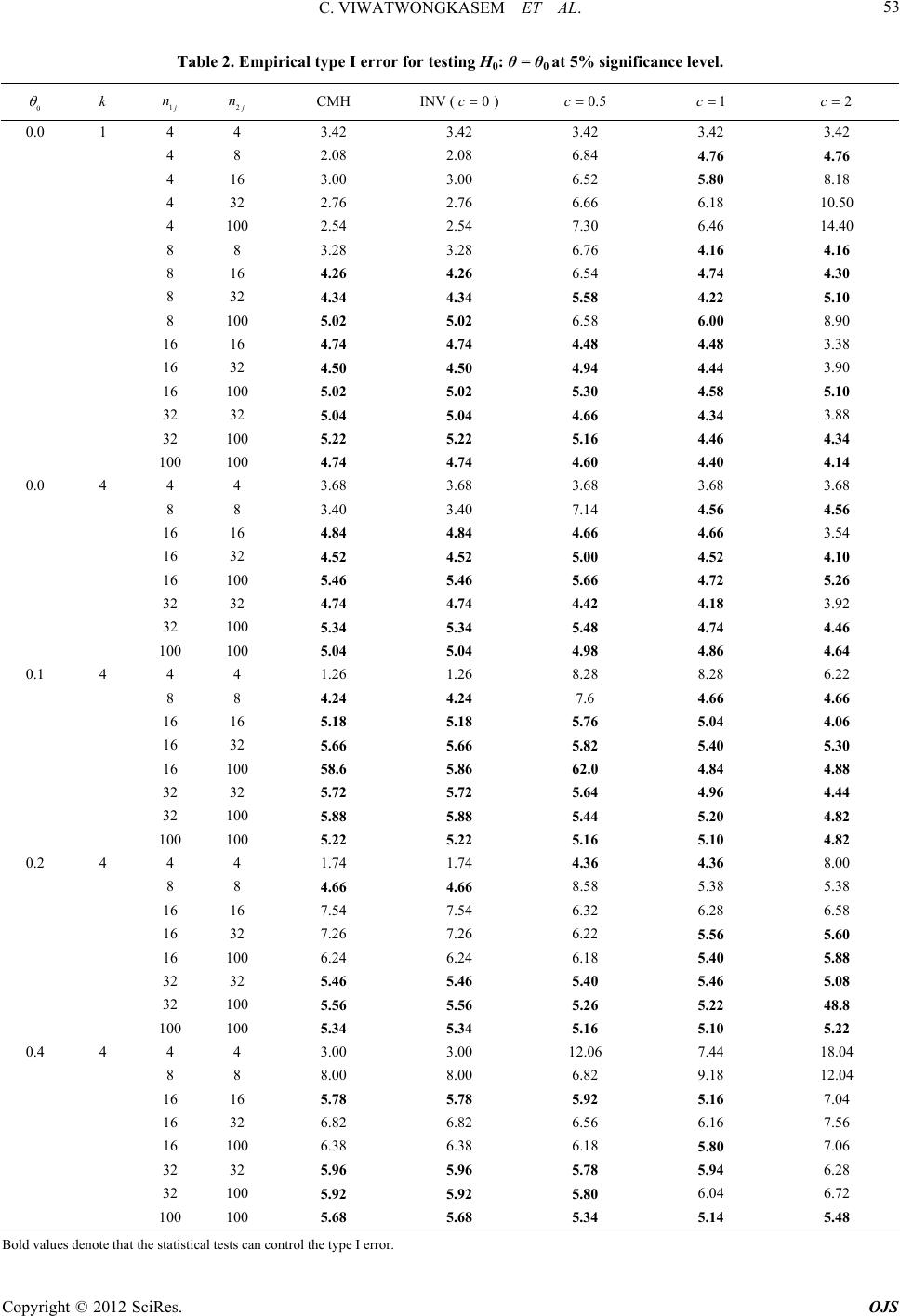

C. VIWATWONGKASEM ET AL.
53
Table 2. Empirical type I error for testing H0: θ = θ0 at 5% significance level.
0

k 1j
n 2j n CMH INV (0c

) 0.5c

1c 2c

0.0 1 4 4 3.42 3.42 3.42 3.42 3.42
4 8 2.08 2.08 6.84 4.76 4.76
4 16 3.00 3.00 6.52 5.80 8.18
4 32 2.76 2.76 6.66 6.18 10.50
4 100 2.54 2.54 7.30 6.46 14.40
8 8 3.28 3.28 6.76 4.16 4.16
8 16 4.26 4.26 6.54 4.74 4.30
8 32 4.34 4.34 5.58 4.22 5.10
8 100 5.02 5.02 6.58 6.00 8.90
16 16 4.74 4.74 4.48 4.48 3.38
16 32 4.50 4.50 4.94 4.44 3.90
16 100 5.02 5.02 5.30 4.58 5.10
32 32 5.04 5.04 4.66 4.34 3.88
32 100 5.22 5.22 5.16 4.46 4.34
100 100 4.74 4.74 4.60 4.40 4.14
0.0 4 4 4 3.68 3.68 3.68 3.68 3.68
8 8 3.40 3.40 7.14 4.56 4.56
16 16 4.84 4.84 4.66 4.66 3.54
16 32 4.52 4.52 5.00 4.52 4.10
16 100 5.46 5.46 5.66 4.72 5.26
32 32 4.74 4.74 4.42 4.18 3.92
32 100 5.34 5.34 5.48 4.74 4.46
100 100 5.04 5.04 4.98 4.86 4.64
0.1 4 4 4 1.26 1.26 8.28 8.28 6.22
8 8 4.24 4.24 7.6 4.66 4.66
16 16 5.18 5.18 5.76 5.04 4.06
16 32 5.66 5.66 5.82 5.40 5.30
16 100 5.86 5.86 6.20 4.84 4.88
32 32 5.72 5.72 5.64 4.96 4.44
32 100 5.88 5.88 5.44 5.20 4.82
100 100 5.22 5.22 5.16 5.10 4.82
0.2 4 4 4 1.74 1.74 4.36 4.36 8.00
8 8 4.66 4.66 8.58 5.38 5.38
16 16 7.54 7.54 6.32 6.28 6.58
16 32 7.26 7.26 6.22 5.56 5.60
16 100 6.24 6.24 6.18 5.40 5.88
32 32 5.46 5.46 5.40 5.46 5.08
32 100 5.56 5.56 5.26 5.22 4.88
100 100 5.34 5.34 5.16 5.10 5.22
0.4 4 4 4 3.00 3.00 12.06 7.44 18.04
8 8 8.00 8.00 6.82 9.18 12.04
16 16 5.78 5.78 5.92 5.16 7.04
16 32 6.82 6.82 6.56 6.16 7.56
16 100 6.38 6.38 6.18 5.80 7.06
32 32 5.96 5.96 5.78 5.94 6.28
32 100 5.92 5.92 5.80 6.04 6.72
100 100 5.68 5.68 5.34 5.14 5.48
Bold values denote that the statistical tests can co ntrol the type I error.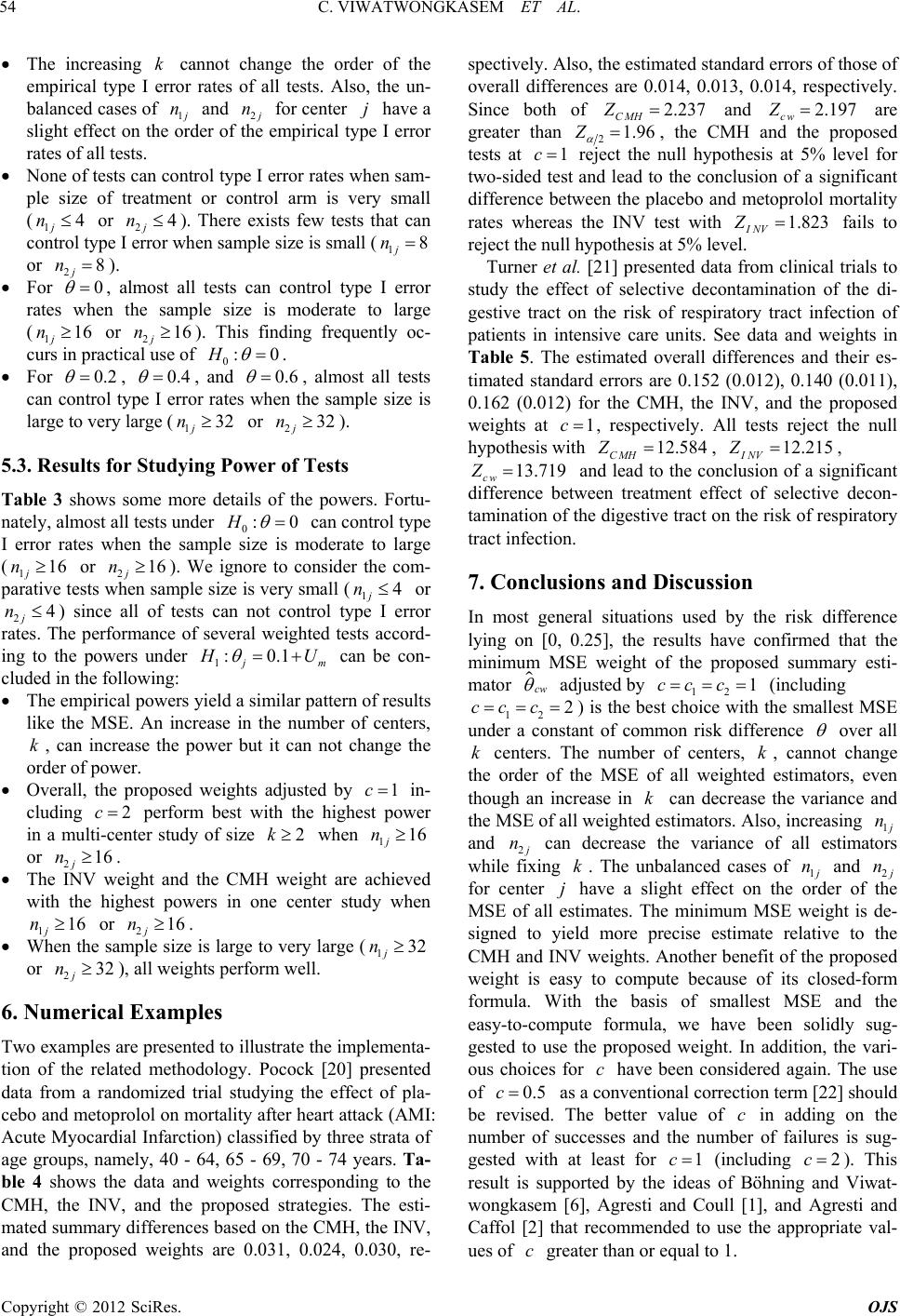

C. VIWATWONGKASEM ET AL.
54
 The increasing k cannot change the order of the
empirical type I error rates of all tests. Also, the un-
balanced cases of 1j n and 2j n for center j have a
slight effect on the order of the empirical type I error
rates of all tests.
 None of tests can control type I error rates when sam-
ple size of treatment or control arm is very small
(14
j
n or 24
j
n). There exists few tests that can
control type I error when sample size is small (18
j
n

or 28
j
n).
 For 0

, almost all tests can control type I error
rates when the sample size is moderate to large
(116
j
n or 216
j
n). This finding frequently oc-
curs in practical use of 0:0H

.
 For 0.2

, 0.4

, and 0.6

, almost all tests
can control type I error rates when the sample size is
large to very large (132
j
n or 232
j
n).
5.3. Results for Studying Power of Tests
Table 3 shows some more details of the powers. Fortu-
nately, almost all tests under 0:0H

 can control type
I error rates when the sample size is moderate to large
(116
j
n or 216
j
n). We ignore to consider the com-
parative tests when sample size is very small (14
j
n

or
24 j
n) since all of tests can not control type I error
rates. The performance of several weighted tests accord-
ing to the powers under 1:0.1
j
m
H
U

 can be con-
cluded in the following:
 The empirical powers yield a similar pattern of results
like the MSE. An increase in the number of centers,
k, can increase the power but it can not change the
order of power.
 Overall, the proposed weights adjusted by 1c

in-
cluding 2c perform best with the highest power
in a multi-center study of size 2k when 116
j
n
or 216
j
n.
 The INV weight and the CMH weight are achieved
with the highest powers in one center study when
116 j
n or 216
j
n.
 When the sample size is large to very large (132
j
n
or 232
j
n), all weights perform well.
6. Numerical Examples
Two examples are presented to illustrate the implementa-
tion of the related methodology. Pocock [20] presented
data from a randomized trial studying the effect of pla-
cebo and metoprolol on mortality after heart attack (AMI:
Acute Myocardial Infarction) classified by three strata of
age groups, namely, 40 - 64, 65 - 69, 70 - 74 years. Ta-
ble 4 shows the data and weights corresponding to the
CMH, the INV, and the proposed strategies. The esti-
mated summary differences based on the CMH, the INV,
and the proposed weights are 0.031, 0.024, 0.030, re-
spectively. Also, the estimated standard errors of those of
overall differences are 0.014, 0.013, 0.014, respectively.
Since both of 2.237
CMH
Z

and 2.197
cw
Z are
greater than 21.96Z


, the CMH and the proposed
tests at 1c

reject the null hypothesis at 5% level for
two-sided test and lead to the conclusion of a significant
difference between the placebo and metoprolol mortality
rates whereas the INV test with 1.823
INV
Z fails to
reject the null hypothesis at 5% level.
Turner et al. [21] presented data from clinical trials to
study the effect of selective decontamination of the di-
gestive tract on the risk of respiratory tract infection of
patients in intensive care units. See data and weights in
Table 5. The estimated overall differences and their es-
timated standard errors are 0.152 (0.012), 0.140 (0.011),
0.162 (0.012) for the CMH, the INV, and the proposed
weights at 1c

, respectively. All tests reject the null
hypothesis with 12.584
CMH
Z

, 12.215
INV
Z,
13.719
cw
Z

and lead to the conclusion of a significant
difference between treatment effect of selective decon-
tamination of the digestive tract on the risk of respiratory
tract infection.
7. Conclusions and Discussion
In most general situations used by the risk difference
lying on [0, 0.25], the results have confirmed that the
minimum MSE weight of the proposed summary esti-
mator

cw

adjusted by 12 1cc c

 (including
12
2cc c

) is the best choice with the smallest MSE
under a constant of common risk difference

over all
k centers. The number of centers, k, cannot change
the order of the MSE of all weighted estimators, even
though an increase in k can decrease the variance and
the MSE of all weighted estimators. Also, increasing 1
j
n
and 2
j
n can decrease the variance of all estimators
while fixing k. The unbalanced cases of 1
j
n and 2
j
n
for center j have a slight effect on the order of the
MSE of all estimates. The minimum MSE weight is de-
signed to yield more precise estimate relative to the
CMH and INV weights. Another benefit of the proposed
weight is easy to compute because of its closed-form
formula. With the basis of smallest MSE and the
easy-to-compute formula, we have been solidly sug-
gested to use the proposed weight. In addition, the vari-
ous choices for c have been considered again. The use
of 0.5c

as a conventional correction term [22] should
be revised. The better value of c in adding on the
number of successes and the number of failures is sug-
gested with at least for 1c (including 2c

). This
result is supported by the ideas of Böhning and Viwat-
wongkasem [6], Agresti and Coull [1], and Agresti and
Caffol [2] that recommended to use the appropriate val-
ues of c greater than or equal to 1.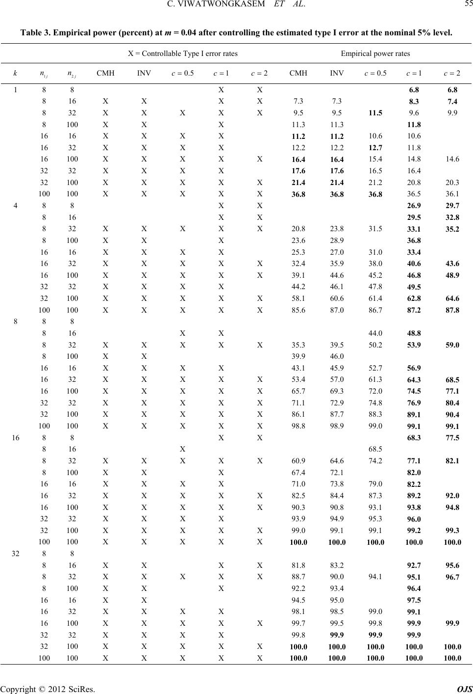

C. VIWATWONGKASEM ET AL.
55
Table 3. Empirical power (percent) at m = 0.04 after controlling the estimated type I error at the nominal 5% level.
X = Controllable Type I error rates Empirical power rates
k 1j
n 2j n CMH INV 0.5c1c

2c

CMH INV 0.5c 1c 2c

1 8 8 X X 6.8 6.8
8 16 X X X X 7.3 7.3 8.3 7.4
8 32 X X X X X 9.5 9.5 11.5 9.6 9.9
8 100 X X X 11.3 11.3 11.8
16 16 X X X X 11.2 11.2 10.6 10.6
16 32 X X X X 12.2 12.2
12.7 11.8
16 100 X X X X X 16.4 16.4 15.4 14.8 14.6
32 32 X X X X 17.6 17.6 16.5 16.4
32 100 X X X X X
21.4 21.4 21.2 20.8 20.3
100 100 X X X X X
36.8 36.8 36.8 36.5 36.1
4 8 8 X X 26.9 29.7
8 16 X X 29.5 32.8
8 32 X X X X X 20.8 23.8 31.5 33.1 35.2
8 100 X X X 23.6 28.9 36.8
16 16 X X X X 25.3 27.0 31.0
33.4
16 32 X X X X X 32.4 35.9 38.0
40.6 43.6
16 100 X X X X X 39.1 44.6 45.2
46.8 48.9
32 32 X X X X 44.2 46.1 47.8 49.5
32 100 X X X X X 58.1 60.6 61.4 62.8 64.6
100 100 X X X X X 85.6 87.0 86.7
87.2 87.8
8 8 8
8 16 X X 44.0 48.8
8 32 X X X X X 35.3 39.5 50.2
53.9 59.0
8 100 X X 39.9 46.0
16 16 X X X X 43.1 45.9 52.7
56.9
16 32 X X X X X 53.4 57.0 61.3
64.3 68.5
16 100 X X X X X 65.7 69.3 72.0 74.5 77.1
32 32 X X X X X 71.1 72.9 74.8 76.9 80.4
32 100 X X X X X 86.1 87.7 88.3
89.1 90.4
100 100 X X X X X 98.8 98.9 99.0 99.1 99.1
16 8 8 X X 68.3 77.5
8 16 X 68.5
8 32 X X X X X 60.9 64.6 74.2 77.1 82.1
8 100 X X X 67.4 72.1
82.0
16 16 X X X X 71.0 73.8 79.0 82.2
16 32 X X X X X 82.5 84.4 87.3 89.2 92.0
16 100 X X X X X 90.3 90.8 93.1
93.8 94.8
32 32 X X X X 93.9 94.9 95.3 96.0
32 100 X X X X X 99.0 99.1 99.1 99.2 99.3
100 100 X X X X X
100.0 100.0 100.0 100.0 100.0
32 8 8
8 16 X X X X 81.8 83.2 92.7 95.6
8 32 X X X X X 88.7 90.0 94.1 95.1 96.7
8 100 X X X 92.2 93.4 96.4
16 16 X X 94.5 95.0 97.5
16 32 X X X X 98.1 98.5 99.0 99.1
16 100 X X X X X 99.7 99.5 99.8
99.9 99.9
32 32 X X X X 99.8 99.9 99.9 99.9
32 100 X X X X X 100.0 100.0 100.0 100.0 100.0
100 100 X X X X X
100.0 100.0 100.0 100.0 100.0

C. VIWATWONGKASEM ET AL.
56
Table 4. Mortality data over three strata of age groups following Pocock.
Age Placebo Metoprolol Weights
j
1j
x
1j n 2j
x
2j n

j

CMH INV 1c

40 - 64 26 453 21 464 0.012 0.66 0 .79 0.69
65 - 69 25 174 11 165 0.077 0.24 0 .16 0.25
70 - 74 11 70 8 69 0.041 0.10 0.05 0.06
Table 5. Respiratory tract infections following Turner et al.
Trial Treatment I Treatment II Weights
j 1j
x
1j n 2j
x
2j n

j

CMH INV 1c

1 25 54 7 47 0.314 0.03 0.02 0.02
2 24 41 4 38 0.480 0.02 0.02 0.03
3 37 95 20 96 0.181 0.05 0.03 0.04
4 11 17 1 14 0.576 0.01 0.01 0.01
5 26 49 10 48 0.322 0.03 0.02 0.02
6 13 84 2 101 0.135 0.05 0.07 0.07
7 38 170 12 161 0.149 0.09 0.09 0.09
8 29 60 1 28 0.448 0.02 0.02 0.03
9 9 20 1 19 0.397 0.01 0.01 0.01
10 44 47 22 49 0.487 0.03 0.02 0.03
11 30 160 25 162 0.033 0.08 0.07 0.06
12 40 185 31 200 0.061 0.10 0.08 0.07
13 10 41 9 39 0.013 0.02 0.01 0.01
14 40 185 22 193 0.102 0.10 0.09 0.09
15 4 46 0 45 0.087 0.02 0.06 0.04
16 60 140 31 131 0.192 0.07 0.04 0.05
17 12 75 4 75 0.107 0.04 0.05 0.05
18 42 225 31 220 0.046 0.12 0.11 0.09
19 26 57 7 55 0.329 0.03 0.02 0.03
20 17 92 3 91 0.152 0.05 0.07 0.07
21 23 23 14 25 0.440 0.01 0.01 0.02
22 6 68 3 65 0.042 0.03 0.07 0.05
In terms of type I error estimates, when sample size is
very small (14
j
n or 24
j
n), none of tests can control
type I error rates. In addition, there exists few tests that
can control type I error rates when sample size is small
(18
j
n or 28
j
n). This result is consonant with the
comments of Lui [23] that none of conventional
tests/weights under sparse data is appropriate. This inap-
propriateness under sparse data can cope with the mini-
mum MSE weights from this finding. The further work
to seek some appropriate tests/weights in sparse data
challenges for investigators to develop an innovation or
to improve much more reasonable tests/weights. In gen-
eral results, almost all tests can control type I error rates
when sample size is moderate to large (116
j
n or
216 j
n).
In terms of power, we ignore to evaluate the power
when sample size is very small (14
j
n or 24
j
n

)
because all tests can not control type I error rates. The
results illustrate the same pattern like the MSE. The pro-
posed weights adjusted by 1c including 2c

per-
form best with the highest power in a multi-center study
of size 2k when 116
j
n or 216
j
n. The INV
weight and the CMH weight are achieved with the high-
est powers in one center study when 116
j
n or
216 j
n. When sample size is large to very large
(132
j
n or 232
j
n), all tests perform well. We

C. VIWATWONGKASEM ET AL.
57
strongly recommend to use the minimum MSE weight as
an appropriate choice because of its highest power.
8. Acknowledgements
We would like to thank the editors and the referees for
comments which greatly improved this paper. This study
was partially supported for publication by the China
Medical Board (CMB), Faculty of Public Health, Mahi-
dol University, Bangkok, Thailand.
REFERENCES
[1] A. Agresti and B. A. Coull, “Approximate Is Better than
Exact for Interval Estimation of Binomial Proportions,”
American Statistical Association, Vol. 52, 1998, pp. 119-
126.
[2] A. Agresti and B. Caffo, “Simple and Effective Confi-
dence Intervals for Proportions and Differences of Pro-
portions Result from Adding Two Successes and Two
Failures,” The American Statistician, Vol. 54, No. 4, 2000,
pp. 280-288. doi:10.2307/2685779
[3] B. K. Ghosh, “A Comparison of Some Approximate Con-
fidence Interval for the Binomial Parameter,” Journal of
the American Statistical Association, Vol. 74, No. 368,
1979, pp. 894-900. doi:10.2307/2286420
[4] R. G. Newcombe, “Two-Sided Confidence Intervals for
the Single Proportion: Comparison of Seven Methods,”
Statistics in Medicine, Vol. 17, No. 8, 1998, pp. 857-872.
doi:10.1002/(SICI)1097-0258(19980430)17:8<857::AID-
SIM777>3.0.CO;2-E
[5] R. G. Newcombe, “Interval Estimation for the Difference
between Independent Proportions: Comparison of Eleven
Methods,” Statistics in Medicine, Vol. 17, No. 8, 1998, pp.
873-890.
doi:10.1002/(SICI)1097-0258(19980430)17:8<873::AID-
SIM779>3.0.CO;2-I
[6] D. Böhning and C. Viwatwongkasem, “Revisiting Pro-
portion Estimators,” Statistical Methods in Medical Re-
search, Vol. 14, No. 2, 2005, pp. 147-169.
doi:10.1191/0962280205sm393oa
[7] G. Casella and R. L. Berger, “Statistical Inference,” Dux-
bury Press, Belmont, 1990.
[8] A. E. Taylor and W. R. Mann, “Advanced Calculus,”
John Wiley & Sons, New York, 1972.
[9] K. J. Lui and K. C. Chang, “Testing Homogeneity of Risk
Difference in Stratified Randomized Trials with Non-
compliance,” Computational Statistics and Data Analysis,
Vol. 53, No. 1, 2008, pp. 209-221.
doi:10.1016/j.csda.2008.07.016
[10] W. G. Cochran, “The Combination of Estimates from
Different Experiments,” Biometrics, Vol. 10, No. 1, 1954,
pp. 101-129. doi:10.2307/3001666
[11] W. G. Cochran, “Some Methods for Strengthening the
Common Chi-Square Test,” Biometrics, Vol. 10, No. 4,
1954, pp. 417-451. doi:10.2307/3001616
[12] N. Mantel and W. Haenszel, “Statistical Aspects of the
Analysis of Data from Retrospective Studies of Disease,”
Journal of the National Cancer Institute, Vol. 22, 1959,
pp. 719-748.
[13] J. Sanchez-Meca and F. Marin-Martinez, “Testing the
Significance of a Common Risk Difference in Meta-
Analysis,” Computational Statistics & Data Analysis, Vol.
33, No. 3, 2000, pp. 299-313.
doi:10.1016/S0167-9473(99)00055-9
[14] J. L. Fleiss, “Statistical Methods for Rates and Propor-
tions,” John Wiley & Sons Inc., New York, 1981.
[15] S. R. Lipsitz, K. B. G. Dear, N. M. Laird and G. Molen-
berghs, “Tests for Homogeneity of the Risk Difference
When Data Are Sparse,” Biometrics, Vol. 54, No. 1, 1998,
pp. 148-160. doi:10.2307/2534003
[16] D. G. Kleinbaum, L. L. Kupper and H. Morgenstern,
“Epidemiologic Research: Principles and Quantitative
Methods,” L i f e t i me Le a rni ng P u b l i c a t i o n s, B e lmont , 1982.
[17] D. B. Petitti, “Meta-Analysis, Decision Analysis and
Cost-Effectiveness Analysis: Methods for Quantitative
Synthesis in Medicine,” Oxford Unive rsity Press, Oxford,
1994.
[18] W. G. Cochran, “The Chi-Square Test of Goodness of
Fit,” Annals of Mathematical Statistics, Vol. 23, No. 3,
1952, pp. 315-345. doi:10.1214/aoms/1177729380
[19] K. J. Lui and C. Kelly, “Tests for Homogeneity of the
Risk Ratio in a Series of 2 × 2 Tables,” Statistics in Medi-
cine, Vol. 19, No. 21, 2000, pp. 2919-2932.
doi:10.1002/1097-0258(20001115)19:21<2919::AID-SI
M561>3.0.CO;2-D
[20] S. J. Pocock, “Cl inical Trials: A Practical Approach,” Wiley
Publication, New York, 1997.
[21] R. Tuner, R. Omar, M. Yang, H. Goldstein and S.
Thompson, “A Multilevel Model Framework for Meta-
Analysis of Clinical Trials with Binary Outcome,” Statis-
tics in Medicine, Vol. 19, No. 24, 2000, pp. 3417-3432.
doi:10.1002/1097-0258(20001230)19:24<3417::AID-SI
M614>3.0.CO;2-L
[22] F. Yates, “Contingency Tables Involving Small Numbers
and the Chi-Squared Test,” Journal of the Royal Statisti-
cal Society (Supplement), Vol. 1, 1934, pp. 217-235.
[23] K. J. Lui, “A Simple Test of the Homogeneity of Risk
Difference in Sparse Data: An Application to a Multicen-
ter Study,” Biometrical Journal, Vol. 47, No. 5, 2008, pp.
654-661. doi:10.1002/bimj.200410150
[24] C. A. Rencher, “Linear Models in Statistics,” Wiley Se-
ries in Probability and Mathematical Statistics, New York,
2000.
[25] A. Sen and M. Srivastava, “Regression Analysis: Theory,
Methods, and Applications,” Springer-Verlag, New York,
1990.

C. VIWATWONGKASEM ET AL.
58
Appendix
Under a true common risk difference

over all k
centers (1, 2,,jk), the mean square error of


1
k
cw cj
cj
jf



 i s given by





2
2
1
k
cw cwcj
cj
j
MSEEE f

 


 



To obtain the optimal weights

cj
f
subject to a
constraint that 110
k
cj
jf 
, we form the auxiliary
function

by following Lagrange’s method to seek

cj
f
that minimize

2
11
1
kk
cj
cj cj
jj
Ef f 







2
2
11 1
21
kk k
cj cj
cj cjcj
jj j
Ef Eff 
 

 


 



2
11
2
11
21
kk
cj cj
cj cj
jj
kk
cj
cj cj
jj
Vf Ef
fE f
 





















2
2
11 1
1
kk k
cj cj
cj cjcj
jj j
fV fEf  
 

 


 
Let


cj
j
VV

 and


cj
j
EE

. The partial de-
rivatives with respect to

and cj
f
yield
11
k
cj
j
f




, 1
22
k
cj jcjjj
j
cj
fVfEE
f





 



Setting 0



 and 0
cj
f



, it yields
11
k
cj
jf



12
k
j
cjcj j
j
j
j
E
ffE
VV




 



Solving for

by taking summation on cj
f
, it yields
111 1
1
12
kkk k
j
cjcj j
jjj j
j
j
E
ffE
VV


 
 

 
 

 

 
 
Let 1
11
1
kk
j
jj
j
aV
V




, 1
k
j
j
j
E
bV

, then 2

can
be written as


1
1
2
k
cjj
j
bfE
aa



 
Hence,
1
1
1
k
cjj
kj
j
cjcj j
j
jjj
bfE
E
ffE
VVaVa









 




11
() 1
kk
jcjj cjjcjj
jj
aVfaEfEbfE









1
1
() 1
k
jcjj cjjj
j
k
cj j
j
aVfaEfEaE
bfEb
















11
k
jcjcjjjj
j
aV ffEaEbaEb







Let jj aE b



11
k
j
cjcj jjj
j
aV ffE










11221
j
cjccck kjj
aV ffEfEfE

 
Substitute each of the subscript j and rearrange
terms.
1j; 1111221 33111 () 1
cc cckk
aVEffEf Ef E

  
2j;


112222 233222
1
cccckk
fEaV EffEfE

  
3j;


1132 23333333
... 1
ccc ckk
fEfEaV EffE

   

jk; 112233 ...()1
ckckc kkkkckk
fEfEfEaV Ef

   
It can be written in the matrix form as Hf y, where
111 21311
122 22322
13233 333
123
k
k
k
kkk kkk
aV EEEE
EaVE EE
EEaVEE
EE EaVE

 
 
 














H



 


C. VIWATWONGKASEM ET AL.
59
123 cc cck
f
ff f


f,


123
1 1 1 1k

 
 
y
The matrix H can be illustrated as

 HDte
where
1
2
00
00
00 k
aV
aV
aV






D




,


12
k



t,


12
k EE E
e
The inverse of H is suggested in several textbooks
of linear model such as Rencher [24] and Sen and
Srivastava [25]. It yields

 
11
1
11
1
1






DteD
H=D+te =D+eDt
Therefore,

 
11
11
1





DteD
f=D
yy
+e Dt




1
11
11
1
11
11
1
1
11
22
22 1
1
1
1
1
1(1 )
1
1(1 )
1(1 )
k
mmm
m
k
mmm
m
k
mmm
m
k
mmm
m
kk
kk
mm
VE
V
a
aEV
V
aVE
V
Va
aaEV
V
aV
aE






 
 






















 



 




  




 

 














f




1
1
1
1
1
k
mmm
m
k
m
m
VE
a
V















































Therefore, for the th j center, it yields

1
1
1
1
1
1
(1 )
1
jj
cj
k
mmm
jj m
k
mmm
m
V
fa
VE
V
a
aEV



























 





where 1
11
1
kk
j
jj
j
aV
V




,
1
k
j
j
j
E
bV

, jj
aE b








12
1112 22
112 2
22
cj
jcjc j
jjj j
jj
EEEpp
npcnpc
nc nc
 













12
1112 22
22
112 2
11
22
cj
jcjc j
j
jjjj j
jj
VVVp p
npp npp
nc nc
 



In practice, we have to estimate the adjusted summary
estimator by replacing the sample estimates for the un-
known quantities:
j
E,
j
V, 1
j
p, 2
j
p,

.