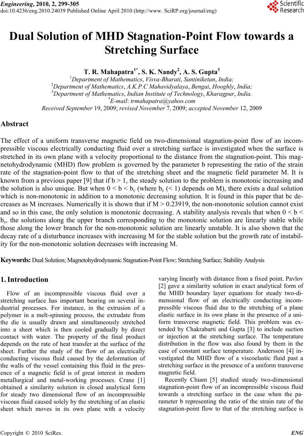Engineering, 2010, 2, 299-305
doi:10.4236/eng.2010.24039 Published Online April 2010 (http://www. SciRP.org/journal/eng)
299
Dual Solution of MHD Stagnation-Point Flow towards a
Stretching Surface
T. R. Mahapatra1*, S. K. Nandy2, A. S. Gupta3
1Department of Mathematics, Visva-Bharati, Santiniketan, India;
2Department of Mathematics, A.K.P.C Mahavidyalaya, Bengai, Hooghly, India;
3Department of Mathematics, Indian Institute of Technology, Kharagpur, India.
*
Received September 19, 2009; revised November 7, 2009; accepted November 12, 2009
Abstract
The effect of a uniform transverse magnetic field on two-dimensional stagnation-point flow of an incom-
pressible viscous electrically conducting fluid over a stretching surface is investigated when the surface is
stretched in its own plane with a velocity proportional to the distance from the stagnation-point. This mag-
netohydrodynamic (MHD) flow problem is governed by the parameter b representing the ratio of the strain
rate of the stagnation-point flow to that of the stretching sheet and the magnetic field parameter M. It is
known from a previous paper [9] that if b > 1, the steady solution to the problem is monotonic increasing and
the solution is also unique. But when 0 < b < bc (where bc (< 1) depends on M), there exists a dual solution
which is non-monotonic in addition to a monotonic decreasing solution. It is found in this paper that bc de-
creases as M increases. Numerically it is shown that if M > 0.23919, the non-monotonic solution cannot exist
and so in this case, the only solution is monotonic decreasing. A stability analysis reveals that when 0 < b <
bc, the solutions along the upper branch corresponding to the monotonic solution are linearly stable while
those along the lower branch for the non-monotonic solution are linearly unstable. It is also shown that the
decay rate of a disturbance increases with increasing M for the stable solution but the growth rate of instabil-
ity for the non-monotonic solution decreases with increasing M.
Keywords: Dual Solution; Magnetohydrodynamic Stagnation-Point Flow; Stretching Surface; Stability Analysis
1. Introduction
Flow of an incompressible viscous fluid over a
stretching surface has important bearing on several in-
dustrial processes. For instance, in the extrusion of a
polymer in a melt-spinning process, the extrudate from
the die is usually drawn and simultaneously stretched
into a sheet which is then cooled gradually by direct
contact with water. The property of the final product
depends on the rate of heat transfer at the surface of the
sheet. Further the study of the flow of an electrically
conducting viscous fluid caused by the deformation of
the walls of the vessel containing this fluid in the pres-
ence of a magnetic field is of great interest in modern
metallurgical and metal-working processes. Crane [1]
obtained a similarity solution in closed analytical form
for steady two dimensional flow of an incompressible
viscous fluid caused solely by the stretching of an elastic
sheet which moves in its own plane with a velocity
varying linearly with distance from a fixed point. Pavlov
[2] gave a similarity solution in exact analytical form of
the MHD boundary layer equations for steady two-di-
mensional flow of an electrically conducting incom-
pressible viscous fluid due to the stretching of a plane
elastic surface in its own plane in the presence of a uni-
form transverse magnetic field. This problem was ex-
tended by Chakrabarti and Gupta [3] to include suction
or injection at the stretching surface. The temperature
distribution in the flow was also found by them in the
case of constant surface temperature. Andersson [4] in-
vestigated the MHD flow of a viscoelastic fluid past a
stretching surface in the presence of a uniform transverse
magnetic field.
Recently Chiam [5] studied steady two-dimensional
stagnation-point flow of an incompressible viscous fluid
towards a stretching surface in the case when the pa-
rameter b representing the ratio of the strain rate of the
stagnation-point flow to that of the stretching surface is

T. R. MAHAPATRA ET AL. 300
equal to unity. By removing this highly restrictive as-
sumption (b = 1), Mahapatra and Gupta [6] analyzed the
steady two dimensional orthogonal stagnation-point flow
of an incompressible viscous fluid towards a stretching
surface in the general case b ≠ 1. They found that the
structure of the boundary layer depends crucially on the
value of b. Temperature distribution in the flow was also
obtained by them. Earlier Mahapatra and Gupta [7] in-
vestigated the steady two- dimensional orthogonal stag-
nation-point flow of an incompressible viscous electri-
cally conducting fluid towards a stretching surface, the
flow being permeated by a uniform transverse magnetic
field. The steady and unsteady equations governing
stagnation-point flow of an electrically nonconducting
incompressible viscous fluid over a stretching surface
along with the existence and uniqueness of the solutions
of these equations were studied by Paullet and Weidman
[8].
In this paper we investigate the dual solution of steady
two-dimensional orthogonal stagnation-point flow of an
incompressible viscous electrically conducting fluid to-
wards a stretching surface in the presence of a uniform
transverse magnetic field. We provided a mathematical
proof in [9] that if b > 1, then the solution of this prob-
lem is monotonic increasing and further this solution is
unique. But for 0 < b < 1, it was shown that there exists a
dual solution which is non-monotonic in addition to a
monotonic decreasing solution. We have found numeri-
cally in this paper that this dual solution exists upto a
certain value of the magnetic parameter M. A linear sta-
bility analysis of these two solutions is also presented.
2. Flow Analysis
Consider the steady two-dimensional stagnation point
flow of an incompressible viscous and electrically con-
ducting fluid permeated by a uniform transverse mag-
netic field towards a flat stretching surface coinciding
with the plane y = 0, the flow being confined to the re-
gion y > 0. Two equal and opposite forces are applied on
the stretching surface along x-axis so that the surface is
stretched with a velocity proportional to the distance
from the stagnation-point which is taken as the origin.
This is shown in Figure 1.
Using boundary layer approximations, the equations
for steady MHD two-dimensional flow are in usual nota-
tion
2
2
11
()
x
uup u
uv
xy xy


 
 
 j,
(1)
1
0
p
y 

 , (2)
where j is the electric current density, B0 is the imposed
uniform magnetic field (acting along the y-direction). In
writing (1), we have neglected the induced magnetic
ou = cx , v = 0
u = ax , v = −ay
Region of non−zero
x
y
Stagnation−poin
t
vorticity
BB B B0000
Figure 1. A sketch of the physical problem.
field since the magnetic Reynolds number RM for the
flow is assumed to be very small. Such an assumption is
justified for the flow of electrically conducting fluids
such as liquid metals e.g., liquid sodium, mercury etc.
[10].
The equation of continuity is
0.
uv
xy


 (3)
Clearly the electric current flows parallel to the z-axis
which is normal to the plane of the flow. Hence by
Ohm’s law
0
0, 0,[],
xy zz
jj jEuB


 (4)
where σ is the electrical conductivity of the fluid which
is assumed constant and Ez is the electric field along
z-axis. It is assumed that the current lines in this
two-dimensional problem close in a manner consistent
with the experiment. Now since the flow is steady,
Maxwell's equation gives

  , (5)
where E is the electric field (which acts parallel to the
z-direction). This gives
0
z
E
x


 and 0
z
E
y


so that Ez is a function of z only.
Since the induced magnetic field is neglected in view
of the assumption RM <<1, electric current in the flow is
determined from Ohm's law and not from =e

B j ,
μe being the magnetic permeability. But the consequence
0
j


0
of this equation must be satisfied [10]. Noting
that the physical variables are functions of x and y,
j

 then gives from (4), Ez = constant. Thus using
(4), we find from (1),

T. R. MAHAPATRA ET AL.301
2
2
2
00
1
.
z
uup u
uv
xy xy
Bu BE




 
 
 

(6)
Since from (2), the pressure p is a function of x only,
the pressure gradient p
x

 can now be obtained from (6)
in the inviscid region as
2
00
1() ,
z
BU BE pdU
Ux
xdx


 
 
(7)
where U(x) is the free stream velocity and use is made
of the fact that Ez is constant. Hence eliminating p
x


from (6) and (7), we get
2 2
0
2()
B uudU u
uvU Uu
xy dxy


 
 
 .
,
(8)
We note that the electric field does not directly affect
the boundary layer equation although it has an influence
on the relation between the free stream velocity and the
pressure distribution given by (7).
Thus the governing equations for the velocity compo-
nents u and v are (3) and (8). The boundary conditions
are
,0 0
() ,
ucxvaty
uUxaxv ay
 
 
(9)
,asy  (10)
where a and c are positive constants. Under the similarity
transformation
1
'2
12
(),( )(),
(/) ,
ucxFvc F
yc





(11)
where a prime denotes derivative with respect to the
similarity variable η, we find that (3) is identically satis-
fied.
Substitution of (11) in (8) then gives
2
''''' '
2'2 2
()() ()()
() 0,
FFFF
MFMbb

 



(12)
where b = a/c and M is the dimensionless magnetic pa-
rameter .
1/ 2
0(/ )Bc

The boundary conditions for (12) then follow from (9)
and (10) as
''
(0)0,(0)1,( ).
F
FFb
,
''
(13)
A detailed proof of the uniqueness of the solution for
the same problem for an electrically non-conducting (M
= 0) fluid was given by Paullet and Weidman [8]. Sub-
sequently the present authors [9] proved the uniqueness
of the solution for an electrically conducting fluid in the
presence of a magnetic field (M ≠ 0) using a similar ap-
proach as that in [8]. In [9] we have shown that if b > 1,
the solution of the boundary value problem (BVP) given
by (12) and (13) is monotonic increasing for all magnetic
parameter M and further this solution is unique. But if 0
< b < 1, there is a dual solution to the above BVP, which
is non-monotonic in addition to a solution which is
monotonic decreasing. Note that when b = 1, the above
BVP admits of the exact solution F(η) = η, which is the
inviscid solution near the stretching surface as found by
Mahapatra and Gupta [7]. However this solution is not
frictionless in a strict sense because in this case the fric-
tion is uniformly distributed and does not therefore affect
the motion.
3. Numerical Solution
Since there is no general analytical solution of the
non-linear differential equation (12) with the boundary
conditions (13) for the case b ≠ 1, so this system is
solved numerically by an efficient shooting method for
different values of M and b. To do this, we first trans-
form the non-linear differential equation (12) to a system
of three first order differential equations as:
''
1223
'22 2
3213 2
,,
()
yyyy
yyyyMybb

  (14)
where '
12 3
(),(),()yF yFyF
 
  and a prime
denotes differentiation with respect to the independent
variable η.
The boundary conditions (13) become
12
2
0, 10,
.
yyat
ybas





(15)
The values of y1 and y2 are given at the starting point η
= 0. But the value of y2 as η→ ∞ is replaced by y2=b at a
finite value η= η∞ to be determined later. The value of y3
at η = 0 is guessed in order to initiate the integration
scheme. Starting from the given values of y1 and y2 at η
= 0 and the guessed value of y3 at η = 0, we integrate the
first order equations (14) by using a fourth-order
Runge-Kutta method up to the end-point η = η∞. The
computed value of y2 at η = η∞ is then compared with y2
= b. The absolute difference between this computed
value and b should be as small as possible. To this end
we use a Newton-Raphson iteration procedure to assure
quadratic convergence of the iterations. The value of η∞
is then increased till y2 attains the value b asymptotically.
4. Dual Solution of MHD Stagnation-Point
Flow
Our numerical results reveal that for 0 < b < 1, in addi-
tion to a monotonic decreasing solution which was al-

T. R. MAHAPATRA ET AL. 302
ready found by Mahapatra and Gupta [7], there exists a
dual solution which is non-monotonic. We have found
that in the absence of magnetic field (M = 0), the
non-monotonic solution exists in the range 0 < b ≤
0.16906. This result in the nonmagnetic case (M = 0) was
also obtained in [8]. For M = 0.1, the dual solution exists
in the range 0 < b ≤ 0.14845, and for M = 0.2, such solu-
tion is found in the range 0 < b ≤ 0.08234. Numerically
we have found that when M ≤ 0.23919, the non-
monotonic solution exists in the range 0 < b <1. Thus we
see that as M increases, the range of b (such that 0 < b <1)
for which the dual (i.e., non-monotonic) solution exists
progressively decreases. The novel result which emerges
from the analysis is that when M > 0.23919, there is no
dual solution in the range 0 < b < 1 and the solution in
this range is monotonic decreasing and unique.
Figure 2 gives the variation of the dimensionless
skin-friction coefficient F''(0) with b for several values of
M. Here the upper branch corresponds to the monotonic
solution while the lower branch corresponds to the non-
monotonic one. It can be seen that for the monotonic
solution, |F''(0)| increases with increase in M. This re-
sult can be physically explained as follows. It is clear
from the momentum equation (8) that when b < 1 (i.e.,
a<c), the Lorentz force given by the last term is negative
because the stagnation-point velocity U(= ax) is less than
the stretching velocity cx of the sheet so that u > U.
Hence this magnetic force decelerates the flow inside the
boundary layer. Since the velocity of a fluid particle par-
allel to the surface is diminished relative to that of the
stretching surface, the velocity gradient at the surface
increases with increase in the magnetic field B0 (charac-
terized by the magnetic parameter M). This results in
increase in the dimensionless skin-friction coefficients
|F''(0)| with increase in M. Note that the above argument
is valid for the monotonic solution for the velocity dis-
tribution because in this case the velocity inside the
boundary layer decreases monotonically from the surface
velocity cx to ax (since a < c) so that u > U.
Figures 3-5 display self-similar velocity profiles of
F'(η) for different values of M at selected values of b.
The non-monotonic behavior of the velocity distribution
is evident from these figures. It is observed from these
figures that for a fixed value of b, the velocity parallel to
the stretching surface at a point in the boundary layer
decreases with increase in M. From a physical point of
view, this follows from the fact that when b < 1, increase
in M leads to increase in the magnitude of the retarding
Lorentz force acting on the fluid resulting in enhanced
deceleration of the flow.
An interesting result which emerges from this analysis
is that for a given value of M, the skin-friction coefficient
|F''(0)| for the dual solution in the case 0 < b < 1 is not a
monotonic function of b but has a maximum at a par-
ticular value of b (see Figure 2). This result is to be con-
trasted with the corresponding result for the monotonic
Figure 2. Reduced skin friction coefficient F''(0) with b for
several values of M showing the upper and lower curves.
Figure 3. Self-similar velocity profiles (for non-monotonic
solution) for b = 0.02 with different values of M.
Figure 4. Self -similar velocity profiles (for non-monotonic
solution) for b = 0.05 with different values of M.
solution for 0 < b < 1, where |F''(0)| decreases monotoni-
cally with increase in b as shown in Figure 2. Physically
this stems from the fact that for the dual solution, the

T. R. MAHAPATRA ET AL.303
Figure 5. Self -similar velocity profiles (for non-monotonic
solution) for b = 0.08 with different values of M.
self-similar velocity profiles F'(η) are non-monotonic
(see Figures 3-5).
5. Stability Analysis
In order to ascertain which of the two solutions in the
region 0 < b < bc (where as shown above, bc depends on
M), is expected to appear asymptotically, we test the sta-
bility of the above two solutions.
To this end, we consider the unsteady form of the
Equation (8) as
2
2
2
0(),
uuudU
uvU
txydxy
BUu




 
 

u
(16)
together with the equation of continuity (3). We seek the
unsteady similarity solution in the form
1/ 2
1/ 2
(,),( )(,),
(/ ),
ucxfv cf
yc







(17)
where the subscript η denotes partial derivative with re-
spect to η and τ is the dimensionless time ct. Note that
with u and v given above, the equation of continuity (3)
is identically satisfied. Substitution of (17) in (16) then
gives
22 2
20,
f
fffMfMb
bf
 


  (18)
where the subscripts η and τ denote partial derivatives
with respect to η and τ respectively. The boundary condi-
tions are
,0 0
() ,
ucxvaty
uUxaxv ay
 
 
,
(19)
.asy  (20)
In terms of f(η,τ), these conditions are
(0,)0,(0,)1,(,).
f
ff

b



 (21)
Following Merkin [11], we put
(,) ()(),fFeg

 

 (22)
where F(η) satisfies (12) subject to (13) and corresponds
to the steady state solution. Further g(η) and all its de-
rivatives are assumed small compared with the steady
solution F(η) and its derivatives. Such an assumption is
made because we are studying the linear stability of the
basic flow F(η) so that the disturbance g(η) is small, γ
being the growth (or decay) rate of the disturbance.
Substituting (22) in (18) and linearizing, we get
''''''2 '''
(2 )0.gFg FMgFg    (23)
Here prime denotes derivative with respect to η. The
boundary conditions for g(η) follow from (13), (21) and
(22) as
''
(0) 0,(0) 0,() 0.gg g (24)
Clearly the homogeneous linear Equation (23) subject to
the homogeneous boundary conditions (24) constitutes
an eigenvalue problem with γ as the eigenvalue. Without
loss of generality, we can take g''(0) = 1. Solutions of (23)
and (24) give an infinite set of eigenvalues γ1 < γ2 < γ3
<… If the smallest eigenvalue γ1 is negative, then there is
an initial growth of disturbances and the flow is unstable.
On the other hand, when γ1 is positive, there is an initial
decay and the flow is stable.
Figure 6 shows the variation of the smallest eigen-
value γ1 for the monotonic solutions (corresponding to
upper curves in Figure 2) with b for several values of the
magnetic parameter M. Since γ1 is real and positive for
these curves, it follows that the monotonic solutions are
linearly stable. Further, for a given value of b, γ1 in-
creases with increase in M. Thus we may say that for
these stable solutions, disturbances decay more quickly
with increase in M.
On the other hand, Figure 7 gives a plot of the varia-
tion of the lowest eigenvalue γ1 for the non-monotonic
Figure 6. Plot of lowest eigenvalues γ1 as a function of b for
the upper branch solution with different values of M.

T. R. MAHAPATRA ET AL. 304
Figure 7. Plot of lowest eigenvalues γ1 as a function of b
for the lower branch solution with different values of
M.
solutions (corresponding to lower curves in Figure 2)
with b for several values of M. Since γ1 < 0 for these
curves, it is clear that the non-monotonic solutions are
linearly unstable. Further for a given b, |γ1| decreases
with increase in M for the non-monotonic solutions.
Hence it follows that the growth rate of unstable distur-
bances decreases with increase in M. A physical inter-
pretation of these results is that the magnetic field has a
stabilizing influence on the flow. In fact a magnetic field
exerts something like a viscous drag on an electrically
conducting fluid and also imparts to it some degree of
rigidity. Thus magnetic field can be expected to inhibit
any tendency to instability. Further from an energetic
point of view, a magnetic field is stabilizing since in ad-
dition to the dissipation of energy by viscosity, there is
dissipation of magnetic energy in the form of Joule heat-
ing [12]. Specially, when an electrically conducting fluid
is perturbed in the presence of a magnetic field, the dis-
turbances induced by currents, whose energy is dissi-
pated by Joule heating.
It may be noted that the result that the monotonic solu-
tion is linearly stable and the non-monotonic solution is
linearly unstable in the case of an electrically noncon-
ducting fluid with M = 0 was arrived at earlier in [8]. Our
present stability analysis is based on the approach in [8].
6. Conclusions
An investigation is made of steady two dimensional
MHD stagnation-point flow of an electrically conducting
incompressible viscous fluid over a stretching surface in
the presence of a uniform transverse magnetic field. The
surface is stretched in its own plane with a velocity pro-
portional to the distance from the stagnation-point. The
flow problem is governed by the dimensionless parame-
ter b representing the ratio of the strain-rate of the stag-
nation flow to that of the stretching surface and the
magnetic parameter M. It is shown that in addition to the
monotonic increasing solution (which is unique) for b >
1 earlier found by Mahapatra and Gupta [7], there exist
two solutions in the range 0 < b < bc, where bc(< 1) de-
pends on M. In this range one solution is monotonic in-
creasing whilst the dual solution is non-monotonic. It is
also found numerically that bc decreases with increase in
M and when M > 0.23919, the dual solution does not
exist.
A linear stability analysis of the two solutions in the
range 0 < b < bc reveals that the monotonic decreasing
solution is linearly stable but the non-monotonic solution
is linearly unstable. Further the magnetic field exerts a
stabilizing influence on the flow.
7. Acknowledgements
We thank the referee for his useful comments which en-
abled us in presenting an improved version of the paper.
The work of one of the authors (T.R.M) is supported
under SAP (DRS PHASE II) program of UGC, New
Delhi. One of the authors (A.S.G) acknowledges the fi-
nancial support of Indian National Science Academy,
New Delhi for carrying out this work.
8. References
[1] L. J. Crane, “Flow Past a Stretching Plate,” Zeitschrift für
Angewandte Mathematik und Physik, Vol. 21, 1970, pp.
645-647.
[2] K. B. Pavlov, “Magnetohydrodynamic Flow of an In-
compressible Viscous Fluid Caused by the Deformation
of a Plane Surface,” Magnitnaya Gidrodinamika, Vol. 4,
1974, pp. 146-147.
[3] A. Chakrabarti and A. S. Gupta, “Hydromagnetic Flow
and Heat Transfer over a Stretching Sheet,” Quarterly of
Applied Mathematics, Vol. 37, April 1979, pp. 73-78.
[4] H. I. Andersson, “MHD Flow of a Viscoelastic Fluid Past
a Stretching Surface,” Acta Mechanica, Vol. 95, 1992, pp.
227-230.
[5] T. C. Chiam, “Stagnation-point Flow towards a Stretch-
ing Plate,” Journal of the Physical Society of Japan, Vol.
63, 1994, pp. 2443- 2444.
[6] T. R. Mahapatra and A. S. Gupta, “Heat Transfer in Stag-
nation-point Flow towards a Stretching Sheet,” Heat
Mass Transfer, Vol. 38, 2002, pp. 517-521.
[7] T. R. Mahapatra and A. S. Gupta, “Magnetohydrody-
namic Stagnation-point Flow towards a Stretching Sheet,”
Acta Mechanica, Vol. 152, 2001, pp. 191-196.
[8] J. Paullet and P. Weidman, “Analysis of Stagnation Point
Flow towards a Stretching Sheet,” International Journal
of Non-Linear Mechanics, Vol. 42, No. 9, 2007, pp.
1084-1091.
[9] T. R. Mahapatra, S. K. Nandy, and A. S. Gupta, “Mag-
netohydrodynamic Stagnation-point Flow of a Power-law
Fluid towards a Stretching Surface,” International Jour-

T. R. MAHAPATRA ET AL. 305
nal of Non-Linear Mechanics, Vol. 44, 2009, pp. 123-128.
[10] J. A. Shercliff, “A Textbook of Magnetohydrodynamics,”
Pergamon Press, Oxford, 1965.
[11] J. H. Merkin, “Mixed Convection Boundary Layer Flow
on a Vertical Surface in a Saturated Porous Medium,”
Journal of Engineering Mathematics, Vol. 14, 1980, pp.
301-313.
[12] S. Chandrasekhar, “Hydrodynamic and Hydromagnetic
Stability,” Clarendon Press, Oxford, 1961.