American Journal of Anal yt ical Chemistry, 2011, 2, 53-62
doi:10.4236/ajac.2011.228124 Published Online December 2011 (http://www.SciRP.org/journal/ajac)
Investigation of the Potential of Near Infrared
Spectroscopy for the Detection and Quantification o f
Pesticides in Aqueous Solution
Aoife A. Gowen1,2*, Yutaro Tsuchisaka1, Colm O’Donnell2, Roumiana Tsenkova1
1Biomeasurement Technology Laboratory, Department of Environmental Information and Bioproduction Engineering,
Graduate School of Agricultural Science, Kobe University, Kobe, Japan
2Biosystems Engineering, University College Dublin, Dublin, Ireland
Received November 3, 2011; revised December 11, 2011; accepted December 19, 2011
Abstract
This research investigates the potential of near infrared spectroscopy (NIRS) for the detection and quantifi-
cation of pesticides in aqueous solution. Standard solutions of Alachlor and Atrazine (ranging in concentra-
tion from 1.25 - 100 ppm) were prepared by dilution in a Methanol/water solvent (1:1 methanol/water (v/v)).
Near infrared transmission spectra were obtained in the wavelength region 400 - 2500 nm; however, the
wavelength regions below 1300 nm and above 1900 nm were omitted in subsequent analysis due to the poor
signal repeatability in these regions. Partial least squares analysis was applied for discrimination between
pesticide and solvent and for prediction of pesticide concentration. Limits of detection of 12.6 ppm for
Alachlor and 46.4 ppm for Atrazine were obtained.
Keywords: Pesticide, Aquaphotomics, Nearinfrared
1. Introduction
In order to enhance monitoring of pesticides it is neces-
sary to develop low cost, rapid methods for their detec-
tion which can be integrated into water flow systems [1].
Vibrational spectroscopy comprises a group of methods
that may be applied for monitoring water quality. Among
the broad spectrum of techniques belonging to this fam-
ily, to date Fourier Transform Infrared (FT-IR) and At-
tenuated Total Reflectance (ATR) spectroscopy in the
mid infrared (MIR) wavelength range (2500 - 16,000 nm)
have been developed for contaminant detection in water
[2]. Due to the high absorption of MIR light by water,
these techniques have depended on the use of pre-en-
richment steps such as solid phase microextraction. Me-
thods based on the coating of the ATR crystals with
polymer films with affinity for certain contaminants have
also been demonstrated. One example is a method de-
veloped for pesticide detection employing PVC coated
ATR crystals; in that study, detection limits around 2
ppm were reported for Atrazine and Alachlor [3]. How-
ever, a 15 minute enrichment time followed by 5 min
water wash was required for each measurement. Such
relatively lengthy measurement times rule out the possi-
bility of on-line monitoring.
In the lower wavelength near infrared (NIR) range
(750 - 2500 nm), the absorption coefficient of water is
around 100 to 1000 times less than that in the MIR. This
facilitates greater sample thickness and direct measure-
ment of water samples. In addition, NIR spectroscopy
(NIRS) is ideally suited for rapid online measurements.
However, NIR spectra are more complicated to analyse
than IR spectra due to the combination and overlapping
of vibrational modes present In order to extract useful
information, it is necessary to apply multivariate tech-
niques such as principal components analysis (PCA),
partial least squares regression (PLSR) etc. [4]. Never-
theless, the detection of low concentrations of contami-
nants in aqueous solution has been demonstrated using
NIRS; researchers recently reported the use of NIRS for
prediction of metal concentration in aqueous solutions
using NIR transmission spectroscopy, with reported lim-
its of detection ranging from 10 - 40 ppm [5]. Although
metals do not absorb light in the NIR, their presence is
detectable due to the interaction of metal ions with OH
bonds in water. Aquaphotomics aims to exploit such in-

A. A. GOWEN ET AL. 54
teractions between water and NIR light to extract infor-
mation on the state of aqueous systems [6]. Water is the
main component in numerous biological (and many non
biological) systems; however, its structure is perturbed
by the presence of various components such as salts,
proteins, sugars and other bio molecules. With this in
mind, Aquaphotomics aims to characterize the effect of
various perturbations on water structure using NIR.
Should changes in the water absorbance patterns arising
from various contaminants be sufficiently distinguishable,
the framework of Aquaphotomics shows potential for
contaminant detection in aqueous systems.
The objective of this work is to evaluate the potential
of NIRS and Aquaphotomics for the detection of pesti-
cides directly in aqueous solution. Although researchers
have demonstrated the potential of NIRS for the detec-
tion of pesticide residues on foods [7,8], to our best
knowledge there are no previous studies reporting the
use of NIRS for detecting pesticides directly in aqueous
solution. Alachlor and Atrazine, were selected as test
analytes for this study. During the 1980s, Alachlor was
introduced as a substitute for Atrazine. These two herbi-
cides have subsequently become important in monitoring
of large scale water bodies and are commonly used in
studies on the development of pesticide contamination
detectors [3]. Atrazine, one of the most frequently ap-
plied herbicides in the USA is a triazine pesticide and
Alachlor, a major corn herbicide, is an acetanilide (Fig-
ure 1). The maximum contaminant level of each under
the US EPA Safe Drinking Water Act (SDWA) is 3 and
2 μg/L (3 and 2 parts per billion (ppb)), respectively [9].
2. Materials and Methods
2.1. Sample Preparation
Due to the low solubility of the selected pesticides in
water, working stock solutions at 100 mg·L–1 were pre-
pared by direct dilution in a solvent of 1:1 methanol/
water (v/v) using deionized water from a Milli-Q water
purification system (Millipore, Molsheim, France) [10].
Further dilutions were made by serial dilution in this
solvent to create a series with the following concentra-
tions: 50, 20, 10, 5, 2.5, 1 mg·L–1 (ppm). The dilutions
were made with the same solvent in order to ensure that
changes in the absorbance signal were due to the pesti-
cide and not due to the changing concentration of solvent.
Methanol and standard quantities of Alachlor (catalogue
number: P-102NM-250) and Atrazine (catalogue number:
P-005NM-250) were purchased from Wako Pure Chemi-
cal Industries (Tokyo, Japan).
The experimental work was carried out in three stages.
In the first stage (carried out between Dec 2010 and April
2011), relatively high pesticide concentrations were
tested (5, 10, 50 and 100 ppm). This high range of con-
centrations was examined in order to test the feasibility
of the method. In the secondary stage (carried out be-
tween June and August 2011), lower pesticide concentra-
tions were employed to further test the detection limit of
the proposed method (1.25, 2.5, 5, 10 and 20 ppm). In
the third stage (carried out in November 2011), interme-
diate pesticide concentrations were tested (1.25, 2.5, 5,
10, 25 and 50 ppm). For the first two stages, each ex-
periment was repeated 6 times (twice per day on three
different days), while for the final stage, each experiment
was repeated four times (twice per day on two different
days). The second experimental day for each stage was
chosen as an independent test set, and the calibration
dataset was composed of the remaining data.
2.2. NIR Spectra Collection
Transmittance spectra were acquired using an NIR Sys-
tem 6500 spectrophotometer (Foss NIR-System, Laurel,
USA), fitted with a quartz cuvette with 1 mm optical
path length. Spectra were measured over the wavelength
region of 400 - 2500 nm, in 2 nm steps. The spectral data
were transformed to pseudo-absorbance units (log(1/T),
where T = transmittance). Transmittance spectra of the
samples of different pesticide concentrations were col-
Figure 1. Chemical structure of Atrazine and Alachlor.

A. A. GOWEN ET AL.55
lected in random order at a temperature of 28˚C ± 1˚C.
The temperature of the sample holder was measured after
each spectral acquisition. Five consecutive spectra were
acquired from each sample. In order to monitor any po-
tentially interfering signals, two control measurements
were taken during each experiment. The first control was
a sample of the solvent while the second consisted of
measuring the empty space (air) between the light source
and detector. These controls were measured at the begin-
ning, middle and end of each experiment. The duration
of each experiment was approximately two hours.
2.3. Data Analysis
All data analysis was carried out in Matlab (The Math-
Works, Inc., Natick, MA) using in house functions. A
number of data pre-treatments were applied to the spec-
tra, as follows: mean centering, multiplicative scatter
correction (MSC), extended multiplicative signal correc-
tion (EMSC), 1st and 2nd derivative Savitsky-Golay (SG)
pretreatments and standard normal variate (SNV) pre-
treatment [4]. In order to improve model robustness,
calibration models were made using all 5 consecutive
spectra. These models were then applied to mean of 5
consecutive spectra in the test set.
The EMSC model can be described as follows:
01 2
XbbXbI

  (1)
where X represents an observed spectrum, b0, b1 and b2
are constants, I is the spectrum of an interferent (in prac-
tice multiple interferent terms can be included in the
model),
X
is a reference spectrum (usually the mean)
and ε is the residual. The constant terms can be estimated
by multiple linear regression and a corrected spectrum
ˆ
X
may be calculated by rearranging Equation (1):
02
11
ˆXb bI
X
bb 1
X
b



(2)
The resultant EMSC corrected spectra are orthogonal
to those of the interferents. In our example, 1st principal
component (PC1) spectra of the controls were used as
interferent spectra.
2.3.1. Exploratory Analysis
Principal component analysis (PCA) [4] was used for
exploratory analysis and to examine the wavelength
ranges at which the experiments were most repeatable.
2.3.2. Cl assification
Partial least squares discriminant analysis (PLSDA) [4]
was employed to discriminate between the solvent and
pesticide-containing solutions. The spectra of the solvent
were designated a dummy index of 0 while those of the
pesticide were designated a value of 1. PLS regression
was applied to the data and a threshold was applied to the
subsequent PLS predictions; any predicted value above
the threshold was designated as belonging to class 1
while the converse were designated as belonging to class
0. In order to avoid model overfitting, the method pro-
posed by Gowen et al. was employed [11]. The % correct
classification for each model on the independent test set
was calculated.
2.3.3. Predictive Modelling
Calibration models were built to predict pesticide con-
centration using PLS regression (PLSR) [4]. In order to
avoid model overfitting, the method proposed by Gowen
et al. was employed [11]. After selecting the optimal
number of latent variables for inclusion, root mean
squared error of prediction (RMSEP) was calculated
based on the predictive performance of the model on the
test set. Due to the nonlinear distribution of pesticide
concentrations, a log transformation was also applied;
however, this did not improve the predictive ability of
the models. Therefore only results for predictive models
built using the original units of concentration are re-
ported here.
2.3.4. Limit of Detection Calculation
The limit of detection of the procedure was calculated
using Equation (3) [12]:
LoD = meanblank + 1.645SDblank + 1.645SDlow (3)
Where the subscript blank refers to a sample not con-
taining the pesticide and low refers to a sample contain-
ing a low concentration of the pesticide. In this study, the
spectra of the solvent were used as blank samples, while
spectra of pesticide solutions containing 1.25 - 2.5 ppm
were used as low samples.
2.4. Safety Considerations
Alachlor and Atrazine are hazardous materials and were
handled under standard laboratory safety conditions.
3. Results and Discussion
3.1. Spectra of Pesticide Solutions
The mean log(1/T) spectra of the Atrazine and Alachlor
solutions are plotted in Figure 2. The main features of
these spectra are major absorbance peaks at 1450, 1940
and 2270 nm, and there a significant baseline effect is
evident, which increases with wavelength (Figure 2(a)).
The mean spectra of the Atrazine and Alachlor solutions
re indistinguishable. However, when they are subtracted a

A. A. GOWEN ET AL. 56
Figure 2. (a) Mean (mean of 5 - 100 ppm concentration) spectra of Atrazine and Alachlor solutions; (b) main regions of dif-
ference between pesticide and solvent shown in normalised (root square difference scaled between 0 - 1) difference spectra of
100 ppm pesticide—solvent; (c) main regions of difference between Atrazine and Alachlor shown in difference spectra of
mean Atrazine and Alachlor spectra shown in (a); (d) main regions of difference between Atrazine and Alachlor shown by
subtracting the spectra shown in (b).
from each other (Figure 2(c)), it is evident that the main
regions of difference occur around 1420 and 1900 nm. In
order to further investigate the spectral changes occur-
ring due to the addition of Atrazine or Alachor to the
water/methanol solvent, the average spectrum of the sol-
vent was subtracted from the average spectrum of the
100 ppm pesticide solutions (Figure 2(b)). The root
square of the difference spectra was scaled to the 0 - 1
range to improve clarity and enable comparison of the
spectral regions affected by the addition of pesticides.
The wavelength regions most affected by the addition of
pesticide, for both Alachor and Atrazine, occurred at
1450, 1908, 1974 and 2274 nm. The regions around 1450
and 1908 nm may be attributed to the first overtone and
combination region of OH stretching and bending vibra-
tions (for pure water, these occur within the ranges 1455
- 1476 nm and 1875 - 1910 nm [13]), the 1974 nm region
corresponds to the combination of NH stretching and
bending vibrations and the 2274 nm region is probably
due to CH combination vibrations [14]. When these
spectra are subtracted from each other (Figure 2(d)), it is
evident that the main regions of difference between A-
trazine and Alachlor occur around 1420 and 1900 nm.
These wavelength regions are related to the perturbation

A. A. GOWEN ET AL.57
of the OH stretching and bending combination vibrations
in the solvent.
3.2. Repeatability of Experiments
In order to investigate which wavelength regions would
be most suitable for data modeling, the data was split
into different wavelength ranges, from 700 - 2500 nm in
steps of 300 nm. Principal component analysis (PCA)
was applied to the data for each day/wavelength range
and the 1st PC loadings for each day were compared, as
plotted in Figure 3. The root square value at each wave-
length range is shown to avoid any confusion caused by
sign ambiguity in PC loadings. It can be observed from
the PC1 loadings that the data from the wavelength re-
gion < 1200 nm and greater than 1900 nm is far noisier
than that in the regions in between these wavelengths.
The noise evident at the spectral edges can be related to
the performance of the detector which is generally of
lower efficiency at those wavelength regions. However,
these noise features also arise due to the characteristics
of the sample: the absorbance of the solvent exceeded 2
absorbance units at wavelengths greater than 1900 nm,
due to the high absorption of light in this region. This
indicates that the response of the detector is nonlinear in
this region. It may also be observed that the Alachlor
data showed greater repeatability (top line, Figure 3)
than the Atrazine data (bottom line, Figure 3), especially
in the 1300 - 1600 nm region. The wavelength region
that appeared least noisy and most repeatable was 1300 -
1900 nm. For this reason, subsequent analysis was car-
ried out in the following wavelength ranges: 1300 - 1600,
Figure 3. Root squared First PC loading for PCA applied to raw absorbance data from (a) high concentration Alachlor (top
line) and Atrazine (bottom line) experiments; (b) low concentration Alachlor (top line) and Atrazine (bottom line) experi-
ments, where wavelength range is indic ate d above each plot. Expe rimental day is represented is by colour (red = day 1, blue =
ay 2, green = day 3). d

A. A. GOWEN ET AL. 58
1600 - 1900 and 1300 - 1900 nm. In these regions the
most striking features in the PC1 loadings were a peak
around 1400 nm and another at around 1900nm corre-
sponding to OH bonds in the solvent. Similar observa-
tions can be made for the low concentration experiments,
shown in Figure 3(b).
3.3. High Concentration Experiments
(5 - 100 ppm)
3.3.1. Discrimination of Pesticide and Solvent
The first task of the analysis was to investigate the po-
tential for NIRS to discriminate between the solvent and
samples of solvent containing pesticide. The data in the
1300 - 1900 nm wavelength region were subjected to a
range of spectral pretreatments and calibration models
were constructed as described in Section 2.3.2. In spite
of applying numerous spectral pretreatments to the data,
it was found that raw log(1/T) data was optimal for dis-
crimination between pesticide solutions and solvent (Ta -
ble 1). For the Alachlor dataset, 100% correct classifica-
tion (CC) was achieved by mean centering the raw log
(1/T) data and building the model in the 1600 - 1900 nm
wavelength range, while for the Atrazine dataset, 85%
correct classification (CC) was achieved by mean cen-
tering the raw log (1/T) data and building the model in
the 1300 - 1600 nm wavelength range (although the same
classification performance was achieved by application
of SNV or EMSC pretreatment in the 1600 - 1900 nm
range).
3.3.2. Prediction of Pesticide Concentration
After discriminating the samples according to the pres-
ence or absence of pesticide, the next objective was to
predict the amount of pesticide present. For this purpose,
PLSR was applied. The model performance in terms of
RMSEP on the independent test set for the range of pre-
treatments tested is shown in Table 2. For the Alachlor
dataset, the model resulting in the lowest prediction error
(11.3 ppm) was one built on SNV pretreated and mean
centered data in the 1300 - 1900 nm range. As for the
Atrazine data, the best performing model (RMSEP =
15.7) resulted from the application of second derivative
Savitsky Golay pretreatment (SG2) to data in the 1300 -
1600 nm wavelength range followed by mean centering.
This is the same wavelength range that was optimal for
the classification of Atrazine, as discussed in the previ-
ous section. The poorer performance of prediction mod-
Table 1. Discrimination of pesticide and solvent for “High concentration” (5 - 100 ppm) experiments, where % CC represents
the percentage correct classification of the independent test set and nlv the number of latent variables used in the PLS-DA
model.
1300 - 1600 nm 1600 - 1900 nm 1300 - 1900 nm
Pesticide Pretreatment nlv % CC nlv % CC nlv % CC
Alachlor Raw 10 53.3 11 66.7 10 60
Raw mn 9 73.3 9 100 9 60
SNV 10 53.3 10 60 9 60
SNV mn 9 53.3 9 73.3 8 66.7
SG1 10 53.3 11 60 11 93.3
SG1 mn 9 73.3 11 93.3 10 93.3
SG2 9 60 11 73.3 11 66.7
SG2 mn 9 80 12 93.3 10 93.3
EMSC 10 73.3 9 93.3 9 80
EMSC mn 10 73.3 9 86.7 8 86.7
Atrazine Raw 9 80 9 75 11 60
Raw mn 9 85 9 70 11 60
SNV 8 80 9 85 10 65
SNV mn 8 80 10 60 9 60
SG1 9 80 12 60 11 70
SG1 mn 8 75 11 55 11 75
SG2 8 80 11 85 10 75
SG2 mn 8 80 11 65 10 65
EMSC 9 70 9 70 10 75
EMSC mn 8 70 9 85 10 75

A. A. GOWEN ET AL.59
Table 2. Prediction of pesticide concentration for high concentration (5 - 100 ppm) experiments, where RMSEP represents
the root mean squared error of prediction of the independent test set and nlv the number of latent variables used in the PLSR
model.
1300 - 1600 nm 1600 - 1900 nm 1300 - 1900 nm
Pesticide Pretreatment nlv RMSEP nlv RMSEP nlv RMSEP
Alachlor Raw 8 76.5 9 39.4 8 18.6
Raw mn 6 58.3 8 32.7 6 23.5
SNV 9 42.9 8 51 7 15.2
SNV mn 9 68.8 10 30.8 6 11.3
SG1 10 55.4 9 33.6 11 11.7
SG1 mn 7 85.9 8 43.8 7 63.1
SG2 9 69.4 10 39.5 8 45.7
SG2 mn 8 38.7 9 37.6 8 62.5
EMSC 8 380.9 9 53 7 84
EMSC mn 7 413.9 8 31.9 6 76.3
Atrazine Raw 8 19.4 9 31.7 9 36.2
Raw mn 9 21.9 10 33.6 9 33.3
SNV 8 22.9 9 24.7 8 27
SNV mn 8 22.9 9 29.3 8 26.8
SG1 8 21.9 12 26.3 10 20
SG1 mn 8 18.3 12 27.1 11 18.5
SG2 7 16.1 11 33.5
9 20.7
SG2 mn 8 15.7 11 35.5 9 17.4
EMSC 9 318.8 9 125.7 9 421.4
EMSC mn 9 291.1 9 126.1 9 634.9
els for Atrazine as compared to Alachlor—or both clas-
sification (see previous section) and quantification—is
remarkable. This may be related to the lower repeatabil-
ity of the AT data, as observed in the PC loading plots
(Figure 1).
3.4. Low Concentration Experiments
(1.25 - 20 ppm)
3.4.1. Discrimination of Pesticide and Solvent
Analysis of the high concentration experiments revealed
that RMSEP values of 10 - 15 ppm could be obtained,
indicating the feasibility of the proposed method. Sub-
sequent experiments were carried out to examine the
potential of NIRS for detection of pesticides in lower
concentrations. Similar to the results for the high con-
centration dataset, the best results for discrimination be-
tween pesticide and solvent was achieved using raw log
(1/T) data (Table 3). 100% correct classification was
achieved for the Alachlor dataset with a model built on
mean centered log(1/T) data in the 1300 - 1900 nm
wavelength range. Models built on the 1600 - 1900 nm
range, which was the optimal range for the high concen-
tration Alachlor experiment, performed poorly in this
case, achieving not greater than 71% correct classifica-
tion. This indicates that different mechanisms underlie
the classification model for high and low concentration
datasets and that the first overtone of the OH stretching
and bending vibrations (1300 - 1600 nm) is important for
the prediction of lower concentrations of pesticides. The
best model for the Atrazine dataset was achieved for
mean centered log(1/T) data in the 1300 - 1600 nm range,
with a classification accuracy of 83.3% attainable. In the
case of Atrazine, the 1300 - 1600 nm wavelength region
was optimal for discrimination between pesticide-con-
taining solutions and solvent for both high and low con-
centration datasets.
3.4.2. Prediction of Pesticide Concentration
The optimal calibration model for the prediction of A-
lachlor concentration was built on EMSC pretreated data
in the 1300 - 1600 nm wavelength range, resulting in an
RMSEP of 4.4 ppm, while that for Atrazine was built on
EMSC pretreated data in the wavelength range 1300 -
1900 nm, resulting in an RMSEP of 15 ppm (Table 4).
These low prediction errors indicate the potential of
NIRS for prediction of low concentration of pesticide in
queous solution. In order to examine the potential of a

A. A. GOWEN ET AL. 60
Table 3. Discrimination of pesticide and solvent for low concentration (1.25 - 20 ppm) experiments, where % CC represents
the percentage correct classification of the independent test set and nlv the number of latent variables used in the PLS-DA
model.
1300 - 1600 nm 1600 - 1900 nm 1300 - 1900 nm
Pesticide Pretreatment nlv CC nlv CC nlv CC
Alachlor Raw 10 70.6 13 58.8 11 94.1
Raw mn 9 70.6 14 70.6 11 100
SNV 9 70.6 13 64.7 10 88.2
SNV mn 8 70.6 12 70.6 10 100
SG1 10 70.6 11 64.7 11 76.5
SG1 mn 9 70.6 12 64.7 11 88.2
SG2 10 70.6 12 58.8 10 64.7
SG2 mn 10 76.5 11 58.8 9 64.7
EMSC 10 58.8 13 64.7 8 58.8
EMSC mn 9 64.7 10 52.9 8 58.8
Atrazine Raw 9 72.2 9 72.2 10 72.2
Raw mn 9 83.3 9 72.2 10 72.2
SNV 9 61.1 10 61.1 10 66.7
SNV mn 9 61.1 11 66.7 9 66.7
SG1 9 61.1 11 66.7 11 66.7
SG1 mn 10 66.7 11 61.1 11 66.7
SG2 10 66.7 11 66.7 10 66.7
SG2 mn 10 66.7 11 61.1 10 66.7
EMSC 9 55.6 8 55.6 9 55.6
EMSC mn 9 50 7 61.1 9 66.7
NIRS for detection of pesticides in aqueous solution for a
wider range of concentrations, it was necessary to com-
bine the high and low concentration datasets and to build
models to predict the range of concentrations tested. This
is the topic of the following sections.
3.5. Combined Data (1.25 - 100 ppm)
3.5.1. Discrimination of Pesticide and Solvent
In order to test the feasibility of the method for a wider
range of concentrations, the high (5 - 100 ppm), low
(1.25 - 20 ppm) and intermediate (1.25 - 50 ppm) con-
centration data were combined (Tab le 5). The maximum
achievable classification accuracy for the Alachlor data-
set was 78.8%, achieved by a model built on mean cen-
tered EMSC pretreated data, while that for Atrazine was
72.4%, achieved by a model built on mean centered SG1
data. Again, the Alachlor samples were better classified
than the Atrazine ones. For both of the pesticides, the
1600 - 1900 region was optimal for classification. The
sensitivity of the best model was 0.87 for Alachlor and
0.76 for Atrazine, while the specificity was 0.76 for
Alachlor and 0.59 for Atrazine.
3.5.2. Prediction of Pesticide Concentration
When prediction models were built on the combined data,
the best performing model for prediction of Alachlor
concentration was found for mean centered SG1 pre-
treated data in the 1300 - 1900 nm range, with an RMSEP
of 6.4 ppm achieved, while the best performing model
for prediction of pesticide concentration in the Atrazine
experiments was one built on SNV mean centered data in
the 1300 - 1600 nm range, with an RMSEP of 16.6 ppm
achieved (Table 6). The limit of detection (LOD) achie-
vable by the best model for Alachlor and Atrazine pre-
diction was calculated as 12.6 ppm for Alachlor and 46.4
ppm for Atrazine. These LODs are comparable to those
reported for the detection of metal contamination in
aqueous samples using NIR transmission spectroscopy
(reported as being in the range 10 - 40 ppm) [5], and are
an order of magnitude higher than those reported for
methods employing polymer enrichment combined with
FT-IR spectroscopy in the wavelength range 4 - 16 μm
(approx 2 ppm) [3].
4. Conclusions
The potential of NIRS for detection of pesticides in
aqueous solutions was examined using Alachlor and
Atrazine as test analytes. Calibration models indicated
that the 1300 - 1900 nm wavelength range, including the

A. A. GOWEN ET AL.61
Table 4. Prediction of pesticide concentration for low concentration (1.25 - 20 ppm) experiments, where RMSEP represents
the root mean squared error of prediction of the independent test set and nlv the number of latent variables used in the PLSR
model.
1300 - 1600 nm 1600 - 1900 nm 1300 - 1900 nm
Pesticide Pretreatment nlv RMSEP nlv RMSEP nlv RMSEP
Alachlor Raw 5 11.6 8 14.2 7 15
Raw mn 5 11.6 7 13.9 6 14.4
SNV 4 11.5 7 13.3 6 13.8
SNV mn 4 13.9 6 13.4 5 14.3
SG1 6 13.4 9 14.7 6 14.9
SG1 mn 5 13.2 9 14.3 6 14.5
SG2 6 12.6 7 12.3 7 14.6
SG2 mn 6 13.6 7 13 6 14.5
EMSC 6 4.4 7 17.4 7 30.5
EMSC mn 7 12.7 8 15.8 8 18.2
Atrazine Raw 8 19.8 8 20.2 9 19.6
Raw mn 8 26.6 10 23.4 9 22.8
SNV 7 20.3 8 19.4 8 21.9
SNV mn 7 21.6 8 19.7 8 21.2
SG1 9 22.2 11 21.7 10 21.5
SG1 mn 9 30.4 11 24.8 9 30.6
SG2 8 21.3 11 21.2 10 21.6
SG2 mn 8 24 10 23.4 9 29.5
EMSC 8 18.9 9 58.6 7 15
EMSC mn 9 26.8 9 37.5 10 26.4
Table 5. Discrimination of pesticide and solvent for com-
bined data (1.25 - 100 ppm), where % CC represents the
percentage correct classification of the independent test set
and nlv the number of latent variables used in the PLS-DA
model.
1300 - 16001600 - 1900 1300 - 1900
Pesticide nlv % CCnlv % CC nlv % CC
Alachlor Raw 12 59.6 12 57.7 10 59.6
Raw mn 12 59.6 12 67.3 965.4
SNV 12 57.7 12 61.5 961.5
SNV mn 11 55.8 11 61.5 861.5
SG1 11 59.6 12 51.9 11 65.4
SG1 mn 11 61.5 11 63.5 1075
SG2 11 53.8 13 53.8 12 63.5
SG2 mn 10 57.7 12 63.5 1171.2
EMSC 12 55.8 11 59.6 1150
EMSC mn 11 57.7 11 78.8 10 51.9
Atrazine Raw 9 69 11 70.7 1165.5
Raw mn 9 67.2 12 70.7 11 65.5
SNV 9 62.1 11 69 1069
SNV mn 9 67.2 11 70.7 11 67.2
SG1 10 60.3 12 70.7 12 63.8
SG1 mn 10 62.1 12 72.4 1262.1
SG2 10 63.8 11 62.1 11 67.2
SG2 mn 9 62.1 11 62.1 11 67.2
EMSC 10 63.8 13 55.2 12 53.4
EMSC mn 10 67.2 12 51.7 11 58.6
Table 6. Prediction of pesticide concentration for combined
data (1.25 - 100 ppm), where RMSEP represents the root
mean squared error of prediction of the independent test
set and nlv the number of latent variables used in the PLSR
model.
1300 - 1600 1600 - 1900 1300 - 1900
Pesticide nlv RMSEP nlv RMSEP nlv RMSEP
AlachlorRaw 10 23.5 10 19.5 10 32.8
Raw mn 1023.4 10 17.6 928.1
SNV 1025.8 12 27.2 944.9
SNV mn1025.7 11 27.3 845
SG1 10 23.1 11 21.1 1118.8
SG1 mn 11 23.4 11 12.5 116.4
SG2 926.9 10 23.5 1219
SG2 mn 1025.9 9 22.6 1215.7
EMSC 11 74.2 10 15.6 10 59.7
EMSC mn1082.6 10 15.5 957.2
Atrazine Raw 921.9 10 29.3 922.7
Raw mn 925.3 9 26.9 918.8
SNV 821.1 9 22.3 920.7
SNV mn816.6 8 24 820
SG1 924.7 11 18.9 1121
SG1 mn 924.1 10 19.3 11 18.2
SG2 822 11 27 10 27
SG2 mn 923.9 11 23.4 10 17.9
EMSC 949.3 9 36.5 1061.3
EMSC mn957.5 9 37 1194.3

A. A. GOWEN ET AL. 62
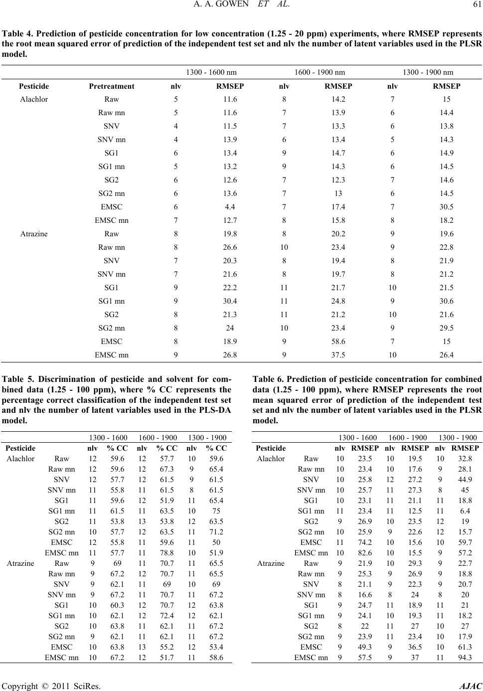
first overtone of the OH stretching and bending modes of
the solvent was important for their identification and
quantification. The proposed method shows potential for
direct measurement of low concentrations of pesticides
in aqueous solution. However, the limits of detection
achieved by analysis of combined low and high concen-
tration experiments (12.6 ppm for Alachlor and 46.4 ppm
for Atrazine) are high compared with the maximum con-
taminant level of each allowed under the SDWA (2 and 3
ppb), respectively. It is also important to note that these
experiments were carried under artificial laboratory con-
ditions. It is well known that the NIR spectrum of aque-
ous samples is susceptible to changes in the environment
(e.g. temperature, humidity) and sample (e.g. pH, turbid-
ity). Therefore, further experiments to test the effect of
such perturbations on predictive ability should be carried
out.
5. Acknowledgements
The first author acknowledges funding from the EU FP7
under the Marie Curie Outgoing International Fellow-
ship.
6. References
[1] ORD, “Technologies and Techniques for Early Warning
Systems to Monitor and Evaluate Drinking Water Quality:
A State-of-the-Art Review,” US Environmental Protec-
tion Agency, Cincinnati, 2005.
[2] A. Gowen, R. Tsenkova, M. Bruen and C. O’Donnell,
“Vibrational Spectroscopy for Analysis of Water for
Human Use and in Aquatic Ecosystems,” Critical Re-
views in Environmental Science and Technology, 2011.
[3] F. Regan, M. Meaney, J. G. Vos, B. D. MacCraith and J.
E. Walsh, “Determination of Pesticides in Water Using
ATR-FTIR Spectroscopy on PVC/Chloroparaffin Coat-
ings,” Analytica Chimica Acta, Vol. 334, No. 1-2, 1996,
pp. 85-92. doi:10.1016/S0003-2670(96)00259-0
[4] H. Martens and M. Martens, “Multivariate Analysis of
Quality: An Introduction,” Wiley, Chichester, 2001.
[5] A. Sakudo, R. Tsenkova, K. Tei, T. Onozuka, K. Ikuta, E.
Yoshimura and T. Onodera, “Comparison of the Vibra-
tion Mode of Metals in HNO3 by a Partial Least-Squares
Regression Analysis of Near-Infrared Spectra,” Biosci-
ence Biotechnology and Biochemistry, Vol. 70, No. 7,
2006, pp. 1578-1583. doi:10.1271/bbb.50619
[6] R. Tsenkova, “Introduction Aquaphotomics: Dynamic
Spectroscopy of Aqueous and Biological Systems De-
scribes Peculiarities of Water,” Journal of Near Infrared
Spectroscopy, Vol. 17, No. 6, 2009, pp. 303-313.
doi:10.1255/jnirs.869
[7] M. T. Sánchez, K. Flores-Rojas, J. E. Guerrero, A. Gar-
rido-Varo and D. Pérez-Marín, “Measurement of Pesti-
cide Residues in Peppers by Near-Infrared Reflectance
Spectroscopy,” Pest Management Science, No. 66, 2010,
p. 580. doi:10.1002/ps.1910
[8] S. Saranwong and S. Kawano, “Rapid Detection of Pesti-
cide Contaminated on Fruit Surface Using NIR-DESIR
Technique: Part II Application on Euparen Detection of
Fresh Tomatoes,” Journal of Near Infrared Spectroscopy,
Vol. 13, 2005, pp. 169-172. doi:10.1255/jnirs.470
[9] http://water.epa.gov/lawsregs/rulesregs/sdwa/
[10] L. L. McConnell, C. P. Rice, C. J. Hapeman, L. Drake-
ford, J. A. Harmon-Fetcho, K. Bialek, M. H. Fulton, A. K.
Leight and G. Allen, “Agricultural Pesticides and Se-
lected Degradation Products in Five Tidal Regions and
the Main Stem of Chesapeake Bay USA,” Environmental
Toxicology and Chemistry, Vol. 26, No. 12, 2007, 2567-
2578. doi:10.1897/06-655.1
[11] A. Gowen, G. Downey, C. Esquerre and C. P. O’Donnel,
“Preventing Over-Fitting in PLS Calibration Models of
NIR Spectroscopy Data Using Regression Coefficients,”
Journal of Chemometrics, Vol. 25, No. 7, 2011, pp. 375-
381. doi:10.1002/cem.1349
[12] D. Armbruster and T. Pry, “Limit of Blank, Limit of De-
tection and Limit of Quantitation,” Clinical Biochemist
Reviews, Vol. 29, 2008, pp. S49-52.
[13] Y. Osaki, “Applications in Chemistry in Near-Infrared
Spectroscopy: Principles, Instruments and Applications,”
In: H. W. Siesler, Y. Ozaki, S. Kawata and H. M. Heise,
Eds., Wiley, Chichester, 2002, p. 182.
[14] L. G. Weyer and S. C. Lo, “Spectra-Structure Correla-
tions in the Near-infrared,” In: J. M. Chalmers and P. R.
Griffiths, Eds., Handbook of Vibrational Spectroscopy,
Wiley, Chichester, Vol. 3, 2002, pp. 1817-1837.