Open Journal of Safety Science and Technology, 2011, 1, 94-100
doi:10.4236/ojsst.2011.13010 Published Online December 2011 (http://www.SciRP.org/journal/ojsst)
Research on Leakage Detection and Analysis of Leakage
Point in the Gas Pipeline System
Zhao Yang1*, Mingliang Liu, Min Shao, Yingjie Ji
Department of T hermal Engin e eri ng , Tianjin University, Tianjin, China
Received June 23, 2011; September 2, 2011; accepted September 15, 2011
Abstract
Recently, with large-scale use of natural gas and massive constructions of gas pipelines, more and more pub-
lic concern is focused on pipeline leakage. The leakage caused by holes on gas pipelines generates economic
losses to gas companies and causes risks to the environment and sometimes accidents. In order to detect and
locate pipeline rupture immediately, the leakage detection method plays a key role in the overall integrity
management in the pipeline system. One of the most important applications of transient simulation is dy-
namic leakage detection. A leakage detection model and the solution were proposed based on the three con-
servation laws in hydromechanics and the state equation, which includes transient simulation model and
volume balance model. Dynamic parameters involved in the model such as pressure, flow and temperature
can be acquired through SCADA (Supervisory Control and Data Acquisition) system. By analyzing the fac-
tors influencing leakage position, we came to a conclusion that leakage and outlet pressure are more impor-
tant parameters compared to the coefficient of frictional resistance and pipeline diameter. The more leakage
increases, the closer leakage point approaches pipeline outlet. Leakage location is closer to outlet when pipe-
line outlet pressure becomes bigger. Experiments were also carried out according to leakage percentage.
Keywords: Leakage Detection, Transient Simulation, Leakage Location, SCADA
1. Introduction
Natural gas is becoming an important energy resource in
China because of its cleanness and high unit-calorie.
Pipeline transportation is one of the most efficient ways
to convey natural gas. Pipeline rupture make sudden
change in pressure, causing economic and environmental
problems without detecting the leakage position and re-
pairing in time [1]. When meeting an ignition source, the
leaked gas may lead to a flame jet, even form a horrible
explosion under proper conditions. The bow-waves of
explosion can kill many lives and destroy buildings. The
traditional way to avoid tragedy is perambulation by
workers. Since the efficiency of perambulation by work-
ers is pretty low, the leakage detection of gas pipeline
with online software plays a key role in the overall integ-
rity management of the pipeline system [2].
With the development of computer technologies and
SCADA (Supervisory Control And Data Acquisition)
system of gas pipeline, various leakage detection meth-
ods based on software are proposed and improved con-
stantly. Pipeline leak detection technologies basically are
divided into two categories: online leak detection system
and discrete leak detection system [3]. According to API
1130, conventional pipeline leak detection systems should
be based on computational pipeline monitoring (CPU)
[4]. A number of pipeline leak detection models have
been implemented on several pipeline systems [5]. Leak-
age detection technologies include the following meth-
ods [6], the volume-mass balance method, the pressure
monitoring method with statistical analysis and/or pat-
tern matching, acoustic monitoring method, the transient
leakage detection method, etc. However, many methods
are hedged in with their shortcomings, which are, long
response time, and incidence of false alarm reporting, etc.
[7].
The transient leakage detection is used to monitor
whether pipeline is in a normal state by establishing the
accurate pipeline model and utilizing perfect numerical
methods. Comparatively speaking, the transient leakage
detection method has the advantages of speediness and
exactness. Gas pipeline leakage detection research based
on transient simulation had begun since the early 1980s
abroad. The transient leakage detection is a major appli-

Z. YANG ET AL.95
cation of transient simulation software, aiming to detect
and locate pipeline rupture immediately. In Japan, gas pi-
peline leakage detection technology using the online si-
mulation method has been used on Niigata-Sendai pipe-
line in 2000. On account of the SCADA system of gas
pipeline hasn’t been developed adequately in China, the
technique was just considered to be primary. In this pa-
per, the factors influencing leakage position were ana-
lyzed.
2. General Description of the Model
2.1. Mathematic Model Base
The flow of gas in pipes can be divided into two situa-
tions. One is that no heat is exchanged between gas in
pipeline and the soil, the other is that the heat is totally
transferred, which means the temperature of gas in pipe-
line is the same as the soil’s [8]. In order to describe the
model conveniently, some assumptions are presented as
follows [9]: 1) The gas flow in pipeline can be described
as a one-dimensional approach, which means the para-
meters are considered to be identical on a section. 2) The
effect of natural gas on external environment is negligi-
ble, that is to say, the soil temperature is constant. 3) The
gas temperature equals to the temperature of pipeline’s
inside wall. 4) The heat transfer process between the soil
and the gas in pipes is steady.
2.2. Transient Simulation Model
As the transient simulation is a kind of numerical method,
accurate equations are had to established to describe the
model. The model is based on solutions of the system of
partial differential equations that describe the conserva-
tion of mass, momentum and energy. State equation is
compulsory. The equations are presented as follows:
Continuity Equation:
() 0 m
x




 (1)
Momentum Equation:
22
() d
d2
mms
gv
x
xd




 




 (2)
Energy Equation:

2
2
2
0
2
2
4d0
d 2
pm
h
kT T
ms
hm mg
xd

 




 



 


 
 



x

(3)
State equation:
p
Z
RT

 (4)
Partial differential equations are converted to ordinary
differential equations with method of characteristics as
shown in Figure 1.
Because Equations (1)-(3) are conservation equations,
the following formula (5) can substitute for them.
AB
C
tx


 (5)
11
1
2
kkkk
iiii1
A
AA A AA
tt t


  

 

(6)
11
1
2
kkkk
iiii
BBBB BB
xx x


  

 
1
(7)
11
1
4
kkkk
iiii
CCCC
C

 
1 (8)
2.3. Volume-Mass Balance Model
In a period of time, the fluid volume loss due to leakage
is equal to the sum of the inlet/outlet volume difference
value and the change in fluid inventory of the pipeline.
The change in fluid inventory of the pipeline influenced
by temperature and pressure include two parts: the varia-
tion of steel pipeline volume and the fluid volume.
The Volume-mass balance equations are presented as
following:
in out
VV VI

  (9)
s
tF
I
II

 (10)

2
01
avg
s
ta
PD
IV T
eE


vg


 




 (11)
0
avg
F
avg
P
IV T
K




 



 (12)
Figure 1. Solving of the transient simulation model.

Z. YANG ET AL. 96
Two independent variables of pressure and tempera-
ture can be acquired on the basis of the volume balance
and the transient simulation, collected through SCADA.
Then average pressure and average temperature in a pe-
riod of time are calculated, which are substituted into
Equations (11) and (12) to get the variation of steel pipe-
line volume
s
I
 caused by temperature and pressure
and volume change of fluid
F
I
 caused by density.
After substituting
s
I
 and
F
I

into Equation (8),
fluid inventory of the pipeline
I
 can be counted. Fi-
nally, by means of Equation (9), leakage volume will be
acquired.
2.4. Leakage Detection System
The leakage detection model includes transient simula-
tion model and volume-mass balance model. When lea-
kage happens, leakage location can be calculated by the
following formulas according to the relation between
flow and pressure, which gas flow in pipeline is in a
steady state [10].

2
11
1
2
2
D

D
XX
fXQ
PP ghh
A

 
D
(13)


2
22
2
2
2
S
XS SX
fLXQ
PP ghh
A
 
 

(14)
In Equations (13) and (14), subscripts D and S denote
outlet and inlet of the pipeline separately, while X repre-
sents leakage location. The parameter h, which stands for
elevation, is really worthy to be discussed. In the high-
pressure transmission and distribution system, the pres-
sure drop due to elevation changes is usually smaller
than that caused by friction by 5%. So, elevation correc-
tions are considered only when the elevation diversifica-
tion exceeds 100 meters every kilometer in the high-
pressure transmission and distribution system. Some-
times, we must add elevation correction in flow calcula-
tion equations [11].
The implemented leakage detection system is illus-
trated in Figure 2. The system contains five modules:
Figure 2. Leakage detection system.
SCADA I/F, data Bass, Transient Simulation, Leakage
Detection, Output.
Our method can make full use of actual data by SC-
ADA (Supervisory Control And Data Acquisition) sys-
tem. It means the accuracy is assured. The weakness is a
mass of sensors are required. Some other leakage detec-
tion methods contain acoustic emission method [12] and
wavelet transform theory [13]. Several weaknesses are
obvious. Acoustic emission method has the limitation of
distance of the sound. The accuracy of wavelet transform
theory is up to the instrument measurement precision.
2.5. SCADA I/F Model
The SCADA system has the function of transferring the
acquired data from a pipeline system to Transient Simu-
lation Model every 30 seconds. This module communi-
cates with SCADA. Dynamic parameters are collected
every 30 seconds, such as pressure, flow and tempera-
ture.
2.6. Transient Simulation Model
Transient flow is simulated utilizing perfect numerical
methods based on actual data. Pressure and temperature
served as independent variables are provided in order to
get average pressure and average temperature. We can
switch the Equations (13) and (14) to different equations
which can be solved with boundary information by virtue
of finite difference method. Then all the parameters of
the gas in the pipeline system can be acquired.
2.7. Leakage Detection
The leakage detection is carried out by comparing the
data acquired through the SCADA system with that by
the Transient Simulation Model. This model could pro-
vide leakage point judgment and prompt warning based
on transient simulation and volume balance.
2.8. Output
To get a supervisory control of the parameters and give
an alarm when something abnormal happens, some out-
puts are necessary. This model includes leakage details,
warning message and parameter values, which includes
pressure, flow, temperature, density, and so on.
3. Factors Influencing Leakage Location
3.1. Leakage Amount and Leakage Location
Suppose pipeline inlet pressure and outlet pressure are
evaluated 1,650,000 Pa and 1,600,000 Pa separately. Inlet

Z. YANG ET AL.97
flux is initially set at 3 m3/s. Leakage percentage ranges
from 0.3% to 93% of the nominal gas flow. Curves on
Figure 3(a) describes the relation between leakage posi-
tion and leakage amount when pipe diameters varies
from 400 mm to 700 mm, while Figure 3(b) shows us
that how the coefficient of frictional resistance influences
leakage position. Obviously, the smaller the pipe diame-
ter is, the further the leakage point is apart from pipeline
inlet under the same other conditions. The trend is simi-
lar to the relationship between the coefficient of fric-
tional resistance and leakage point. However, the curves
based on different pipe diameters and the coefficient of
frictional resistance are so close to each other, which means
these two parameters influence leakage position pretty
slightly. Compared to pipe diameter and the coefficient
of frictional resistance, Figures 3(a) and (b) show that
the leakage amount is a more important parameter.
When outlet flux is larger than 2.8 m3/s, it could
hardly detect whether leakage happens and locate leak-
age position, since even if gas flow down pipeline is in a
normal state, flow loss may be created due to friction.
The more leakage amount increases, the closer leakage
position approaches pipeline outlet. When leakage per-
centage ranges from 0.3% to 33% of the nominal gas
0.00.51.01.52.02.53.0
0
5
10
15
20
25
30
35
leakage point being away from inlet Km
D=400mm
D=500mm
D=600mm
D=700mm
Leakage m3/s
(a)
0.0 0.5 1.0 1.5 2.0 2.5 3.0
0
5
10
15
20
25
30
35
40
Leakage Point Being Away from Inlet Km
f=0.012
f=0.016
f=0.018
f=0.020
Leakage m3/s
(b)
Figure 3. Relation between leakage point and leakage.
flow, leakage location is moving from 36.7 kilometers to
less than 10 kilometers away from pipeline inlet. How-
ever, with the leakage percentage continues growing,
leakage location has little diversification. The leakage
point is always less than 10 kilometers apart from pipe-
line inlet. The reason for the trend of the curve in Figure
4 will be elaborated in next section.
For pipeline DX section, it satisfies the equation
22
2
DX
PP kQ
x
, while for pipeline XS section, it meets
the equation
22
2
XS
PP kQ
Lx

. Therefore, for the same
pipeline, any point pressure can be expressed as Equation
(15).

222
XDDS
X
PPPP
L
 (15)
According to Equation (10) and Figure 4, it is clearly
shows that the further the point is apart from pipeline
inlet, the faster pressure descends. The pressure of the
whole pipeline descends by half in 3/4 length of pipeline
away from inlet [14]. When leakage point is closer to
inlet, the pressure is higher, so differential pressure be-
tween gas and atmosphere is still bigger, and leakage is
even more. It means differential pressure is even bigger
and leakage location is nearer to pipeline inlet when lea-
kage is much more.
3.2. Outlet Pressure and Leakage Location
Suppose that pipeline inlet pressure is initially set at
1,650,000 Pa and inlet flux 3 m3/s. The outlet pressure
ranges from 1,650,000 Pa to 100,000 Pa to guarantee it
higher than atmospheric pressure. The relation between
leakage location and pipeline outlet pressure has been
studied, which is described in Figure 4.
Figure 4. Gas pipeline and pressure changes.

Z. YANG ET AL. 98
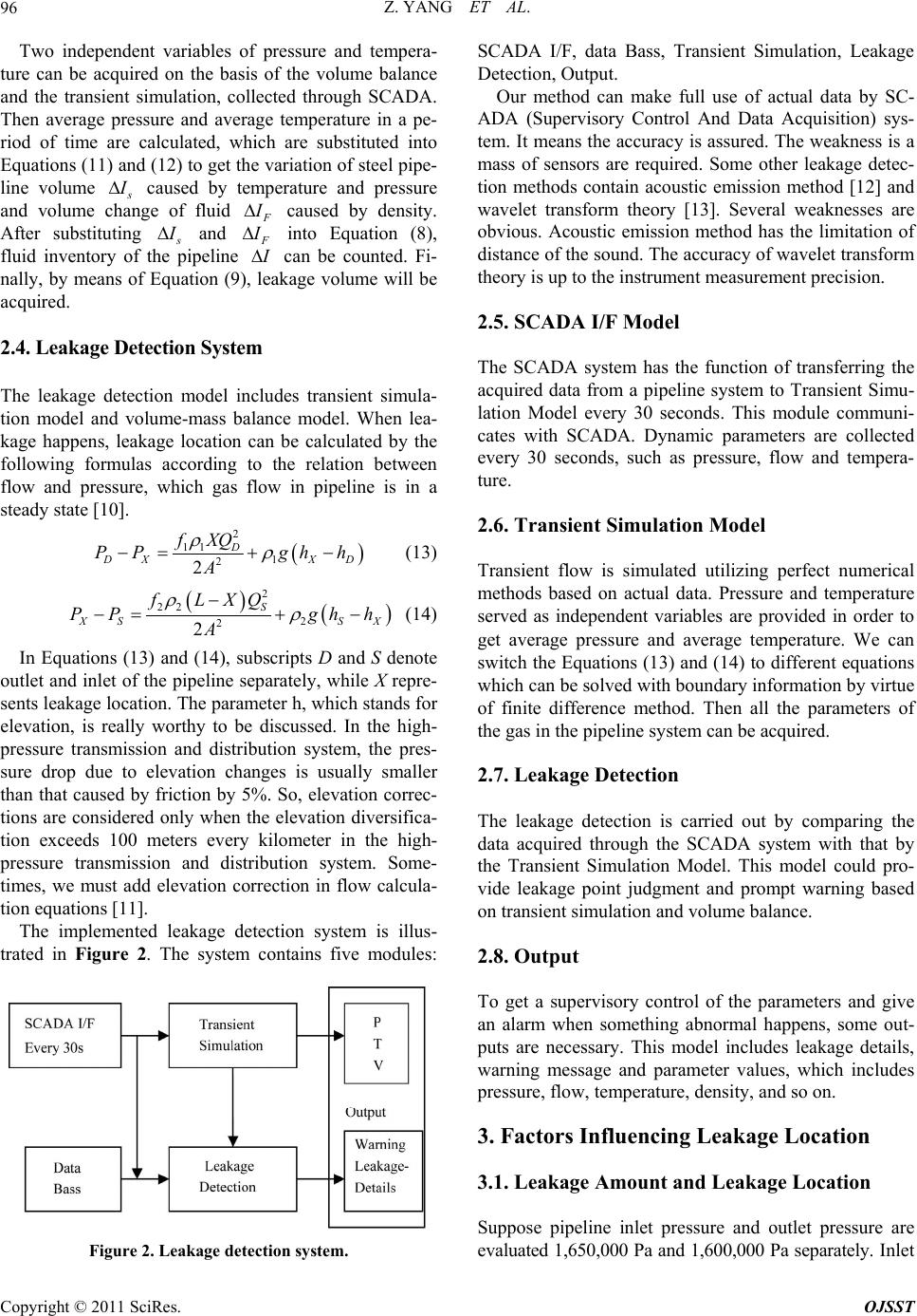
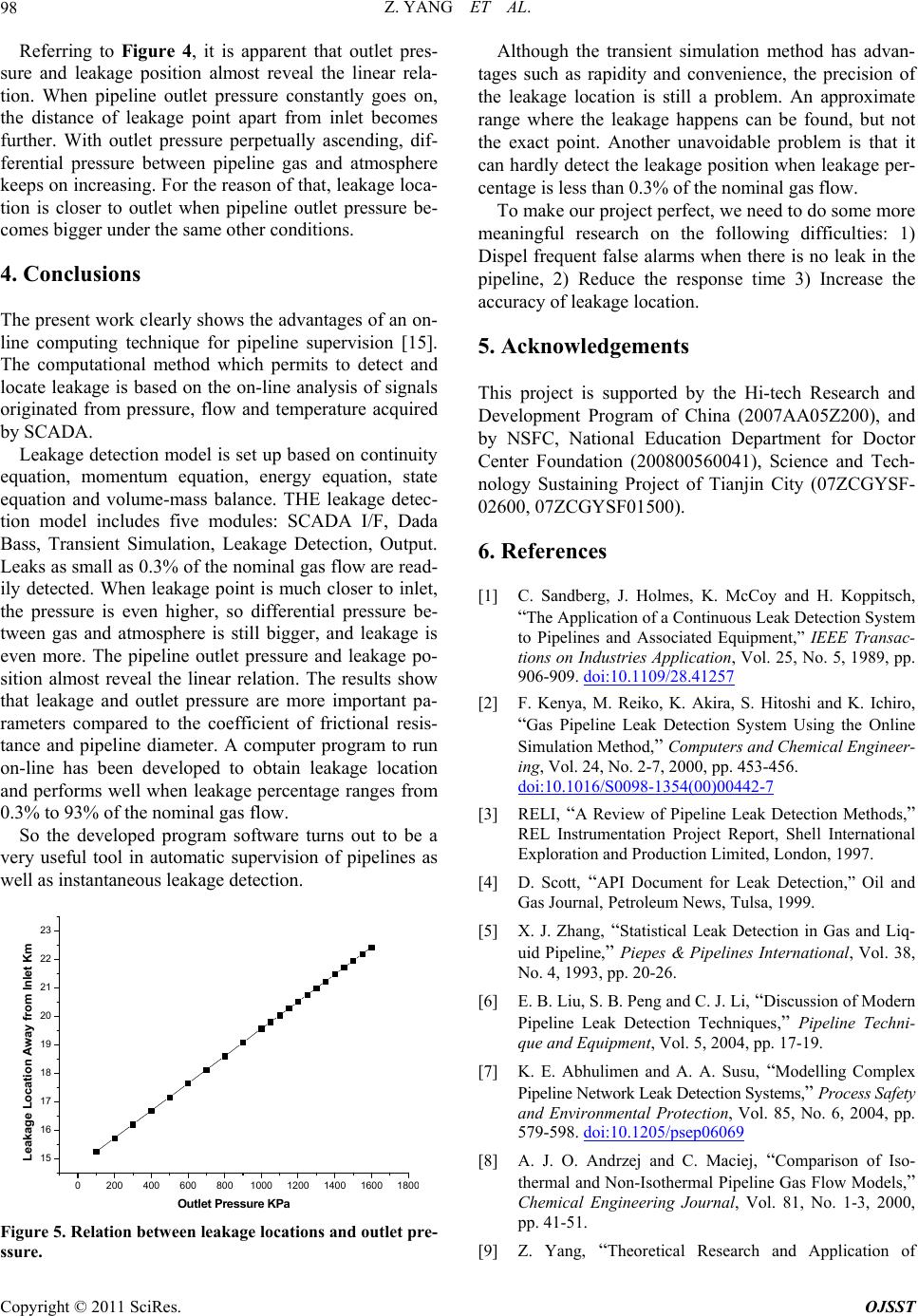
Referring to Figure 4, it is apparent that outlet pres-
sure and leakage position almost reveal the linear rela-
tion. When pipeline outlet pressure constantly goes on,
the distance of leakage point apart from inlet becomes
further. With outlet pressure perpetually ascending, dif-
ferential pressure between pipeline gas and atmosphere
keeps on increasing. For the reason of that, leakage loca-
tion is closer to outlet when pipeline outlet pressure be-
comes bigger under the same other conditions.
4. Conclusions
The present work clearly shows the advantages of an on-
line computing technique for pipeline supervision [15].
The computational method which permits to detect and
locate leakage is based on the on-line analysis of signals
originated from pressure, flow and temperature acquired
by SCADA.
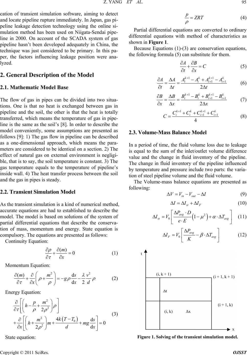
Leakage detection model is set up based on continuity
equation, momentum equation, energy equation, state
equation and volume-mass balance. THE leakage detec-
tion model includes five modules: SCADA I/F, Dada
Bass, Transient Simulation, Leakage Detection, Output.
Leaks as small as 0.3% of the nominal gas flow are read-
ily detected. When leakage point is much closer to inlet,
the pressure is even higher, so differential pressure be-
tween gas and atmosphere is still bigger, and leakage is
even more. The pipeline outlet pressure and leakage po-
sition almost reveal the linear relation. The results show
that leakage and outlet pressure are more important pa-
rameters compared to the coefficient of frictional resis-
tance and pipeline diameter. A computer program to run
on-line has been developed to obtain leakage location
and performs well when leakage percentage ranges from
0.3% to 93% of the nominal gas flow.
So the developed program software turns out to be a
very useful tool in automatic supervision of pipelines as
well as instantaneous leakage detection.
02004006008001000 1200 1400 1600 180
0
15
16
17
18
19
20
21
22
23
Leakage Location Away from Inlet Km
Outlet Pressure KPa
Figure 5. Relation between leakage locations and outlet pre-
ssure.
Although the transient simulation method has advan-
tages such as rapidity and convenience, the precision of
the leakage location is still a problem. An approximate
range where the leakage happens can be found, but not
the exact point. Another unavoidable problem is that it
can hardly detect the leakage position when leakage per-
centage is less than 0.3% of the nominal gas flow.
To make our project perfect, we need to do some more
meaningful research on the following difficulties: 1)
Dispel frequent false alarms when there is no leak in the
pipeline, 2) Reduce the response time 3) Increase the
accuracy of leakage location.
5. Acknowledgements
This project is supported by the Hi-tech Research and
Development Program of China (2007AA05Z200), and
by NSFC, National Education Department for Doctor
Center Foundation (200800560041), Science and Tech-
nology Sustaining Project of Tianjin City (07ZCGYSF-
02600, 07ZCGYSF01500).
6. References
[1] C. Sandberg, J. Holmes, K. McCoy and H. Koppitsch,
“The Application of a Continuous Leak Detection System
to Pipelines and Associated Equipment,” IEEE Transac-
tions on Industries Application, Vol. 25, No. 5, 1989, pp.
906-909. doi:10.1109/28.41257
[2] F. Kenya, M. Reiko, K. Akira, S. Hitoshi and K. Ichiro,
“Gas Pipeline Leak Detection System Using the Online
Simulation Method,” Computers and Chemical Engineer-
ing, Vol. 24, No. 2-7, 2000, pp. 453-456.
doi:10.1016/S0098-1354(00)00442-7
[3] RELI, “A Review of Pipeline Leak Detection Methods,”
REL Instrumentation Project Report, Shell International
Exploration and Production Limited, London, 1997.
[4] D. Scott, “API Document for Leak Detection,” Oil and
Gas Journal, Petroleum News, Tulsa, 1999.
[5] X. J. Zhang, “Statistical Leak Detection in Gas and Liq-
uid Pipeline,” Piepes & Pipelines International, Vol. 38,
No. 4, 1993, pp. 20-26.
[6] E. B. Liu, S. B. Peng and C. J. Li, “Discussion of Modern
Pipeline Leak Detection Techniques,” Pipeline Techni-
que and Equipment, Vol. 5, 2004, pp. 17-19.
[7] K. E. Abhulimen and A. A. Susu, “Modelling Complex
Pipeline Network Leak Detection Systems,” Process Safety
and Environmental Protection, Vol. 85, No. 6, 2004, pp.
579-598. doi:10.1205/psep06069
[8] A. J. O. Andrzej and C. Maciej, “Comparison of Iso-
thermal and Non-Isothermal Pipeline Gas Flow Models,”
Chemical Engineering Journal, Vol. 81, No. 1-3, 2000,
pp. 41-51.
[9] Z. Yang, “Theoretical Research and Application of

Z. YANG ET AL. 99
Steady and Transient Simulation of Gas Network,” Na-
tural Gas Industry Journal, Vol. 26, No. 4, 2006, pp.
105-108.
[10] X. K. Xing, “A Simulation Method of Leakage Detection
in Product Pipeline,” Pipeline Technique and Equipment,
Vol. 3, 2000, pp. 12-14.
[11] Y. J. Li, “Design and Practice of Transmission and Dis-
tribution System,” China Construction Industry Press,
Beijing, 2007, pp. 152-153.
[12] B. Van Hieu, S. Choi, Y. Uk. Kim, Y. Park and T. Jeong
“Wireless Transmission of Acoustic Emission Signals for
Real-Time Monitoring of Leakage in Underground
Pipes”, KSCE Journal of Civil Engineering, Vol. 15, No.
5, 2011, pp. 805-812. doi:10.1007/s12205-011-0899-0
[13] Z. Yang, Z. Xiong and M. Shao, “A New Method of
Leak Location for the Natural Gas Pipeline Based on
Wavelet Analysis,” Energy, Vol. 35, No. 9, 2010, pp. 3814-
3820. doi:10.1016/j.energy.2010.05.034
[14] S. L. Wang and H. J. Zhao, “Design and Management of
Gas Pipeline,” Chemical Industry Press, Beijing, 2006,
pp. 101-103
[15] A. S. Relnaldo, M. B. Clsudio, L. C. Sandra, J. A. F. R.
Pereira, “Pressure Wave Behavior and Leak Detection in
Pipeline,” European Symposium on Computer Aided Pro-
cess Engineering, Vol. 20, Supplement 1, 1996, pp. 491-
496.

Z. YANG ET AL. 100
APPENDIX
Table 1. (Iterative) algorithmic (In %) relative (absolute)
efficiency/gain for f(x) = exp(x).
Items ↓ n→3 6 9
PRE_PFB (f;x)[n] 7.7098 7.97506 8.0614
PRE_PDFBV (f;x)[n] 0.0004 0.00000 0.0000
PRG_PDFBV(f;x)[n] 99.994 100.000 99.999
Table 2. (Iterative) algorithmic (In %) relative (absolute)
efficiency/gain for f(x) = ln(2+x).
Items ↓ n→3 6 9
PRE_PFB (f;x)[n] 5.0970 5.0217 4.9961
PRE_PDFBV (f;x)[ n] 0.0001 0.0000 0.0000
PRG_PDFBV (f;x )[n] 99.996 100.00 99.999
Table 3. (Iterative) algorithmic (In %) relative (absolute)
efficiency/gain for f(x) = sin(2 + x).
Items ↓ n→3 6 9
PRE_PFB (f;x)[n] 5.0404 5.3105 5.4020
PRE_PDFBV (f;x)[n] 0.0004 0.0000 0.0000
PRG_PDFBV (f;x)[n] 99.991 99.999 99.999
Table 4. (Iterative) algorithmic (In %) relative (absolute)
efficiency/gain for f(x) = 10x.
Items ↓ n→3 6 9
PRE_PFB (f;x)[n] 16.112 17.498 17.935
PRE_PDFBV (f;x)[ n] 0.0120 0.0000 0.0000
PRG_PDFBV (f;x )[n] 99.925 99.999 99.999