Applied Mathematics, 2011, 2, 1546-1550
doi:10.4236/am.2011.212220 Published Online December 2011 (http://www.SciRP.org/journal/am)
Test of Generating Function and Estimation of Equivalent
Radius in Some Weapon Systems and Its Stochastic
Simulation
Famei Zheng
School of Mathematical Science, Huaiyin Normal University, Huai’an, China
Received November 16, 2011; revised December 6, 2011; accepted December 14, 2011
Abstract
We discuss three-dimensional uniform distribution and its property in a sphere; give a method of assessing
the tactical and technical indices of cartridge ejection uniformity in some type of weapon systems. Mean-
while we obtain the test of generating function and the estimation of equivalent radius. The uniformity of
distribution is tested and verified with ω2 test method on the basis of stochastic simulation example.
Keywords: Uniform Distribution in a Sphere, Weapon Systems, Generating Function, Equivalent Radius,
Stochastic Simulation
1. Introduction
Uniform distribution is very important in the probability
statistics, many scholars pay attention to it. The follow-
ing questions have been explored: the estimate of inter-
val length about uniform distribution in [a,b] [1,2], the
estimate of regional area about two dimension uniform
distribution in a rectangle [3], the estimate of cuboid
volume about three dimension uniform distribution [4],
the estimate of regional area about two-dimensional uni-
form distribution in a circle [5,6], estimate of radius on
three-dimensional uniform distribution in a sphere [7]. In
addition, many scholars get useful test statistics and limit
theorems [8-12]. In this paper, basing on some articles
[13-18], according to t the indices of cartridge ejection
uniformity in some type of weapon systems, we give the
test of generating function and the estimation of equiva-
lent radius by simulation example.
Definition 1 [7]. If (,,)
X
YZ is three-dimensional
continuous random variable, its probability density func-
tion is
3
0
3,(,,)
4π (, ,)
0(,,)
,
.
x
yz G
R fxyz
x
yz G





(1.1)
where


2222
00
(, ,),0Gxyzxyz RR, then we
call that (,,)
X
YZ obeys uniform distribution in


2222
0
(, ,)GxyzxyzR

, recorded as (X,Y,Z)~U(G).
Give a transformation
0
sin cos
sin sin(0,0π,0 2π)
cos
xr
yr rR
zr

 







(1.2)
The probability density function of three-dimensional
r.v.(,, )R

 is
(, ,)
( ,,)(sincos,sinsin,cos)(, , )
x
yz
hrf rrrr  




(1.3)
in which 0
0,0π,0 2π,rR



(, ,)
(, , )
x
yz
r



 is
Jacobi determinant of the transformation (1.2), and
2
(, ,)
(, , )
sin coscos cossin sin
sinsincos sinsincos
cos sin0
sin
xxx
r
xyzy yy
rr
zzz
r
rr
rr
r
r

 


 





 




 




 (1.4)

F. M. ZHENG1547
Therefore the probability density function of (, , )R


is
2
0
3
0
3sin,0,0 π,0 2π
(, , )4π
0, otherwise
rrR
hr R


 




(1.5)
Theorem 1. If the marginal density functions of
about are
r.v.
(, , )R ,,R 1(),hr 2(),h

3()h

,
then
1)
2
0
3
10
3,0
()
0, otherwise.
rrR
hr R





,
2) 2
1sin ,0π,
() 2
0, otherwise
h






.
3) 3
1,0 2π,
() 2π
0, otherwise.
h







Proof. According to (1.5) and the definition of mar-
ginal density function, we have
π2π
100
22
π2ππ
33
00 0
00
22
33
00
0
()(,, )d d
3sin 3
dd 2πsin d
4π4π
33
2π2,
4π
where 0,
hr hr
rr
RR
rr
RR
rR
 





 


 

00
0
2
2π2π
23
00 00
0
2
30
0
3sin
( )(,, )dddd
4π
3sin 1
2πdsin,
2 4π
where 0π,
RR
R
r
hhrr R
rr
R

r

 



 

 

00
0
2
ππ
33
00 00
0
π
23
0
33
00
00
3sin
( )(,,)dddd
4π
33
dsind 2
3 4π4π
1,
2π
where 02π.
RR
R
r
hhrr R
rr R
RR

1
r

 






 
 
Corolla ry 1 [7]. If r.v.(, , )R

 is defined by (1.5),
then three are independent each other. r.v.,,R
Corollary 2. If is defined by (1.5), the
marginal distribution function of about
are
r.v.
12
(),H
(, , )R
3
(),( )H
r.v.(, , )R
,,R Hr

 , then
3
10
3
0
0
0, 0
() ,0
1,
r
r
H
rr
R
rR
 







R
,
2
0, 0
1
()(1 cos ),0π
2
1, π
H














,
3
0, 0
(),02π
2π
1,2 π
H












.
Proof. According to theorem 1, we can get it easily.
Corollary 3. If ()ER


, 2
()Var R

, then the
probability of cartridges falling into a ball with radius

is about 42.2%, and the probability of cartridges fal-
ling into a sphere with radius

  is about 84.0%.
Proof. By the definition of Mathematical expectation,
we have
0
1
0
3
()()d 4
R
ERrh rrR   
0
(1.6)
00
4
22
10
3
00
0
33
()()dd 5
RR
r
ERrh rrrR
R

 2
 (1.7)
then
22222
00
39 3
()()()51680 DRERE RRRR    
2
0
and 0
15
20 R
 , then the probability of cartridges fal-
ling into a sphere with radius

is about

11 10
3
() ()42.2%
4
HHERHR




 (1.8)
then the probability of cartridges falling into a sphere
with radius



is about

1100
31584.0%
420
HHRR


 



(1.9)
2. Test of Generating Distribution Function
Usually there are 2

test method, 2

test method and
Cole Moge Rove test method (K test method) [17] to test
distribution function. Here, we use 2

test method, we
want to know the sub-sample is uniform distribution or
not. Because the locations of any cartridges are ascer-
tained by three-dimensional , so we should r.v.(, ,)R

F. M. ZHENG 1548
))test them one by one, test 1, ~(RHr 2 ~(H

,
3
~(H)

. We give testing hypotheses 0
H
00
():()
H
Fx x


where ()
F
x is generating distribution function, 0()
x

is known distribution function, and 0()
x

is the deriva-
tive of 0()
x

,,yy
.
Tests for generating function should be independent,
(1)(2)() is the sequent sub-sample of the test,
under hypotheses
,
n
y
0
H
is correct, the statistic
2
21



2
1
1
12
n
i
n



0(
)
() 2
i
i
y
nn

  (2.1)
is Smirnov distribution. For the given confidence level

,
according to the Table 10 in [17], we obtain the boundary
value z

of 2 n

, in which 2 (Pn )

z

  . Then
is rejection region of the hypotheses 0 (,)z


H
, when
2
nz

 , we reject 0
H
, if 2 nz

 , we should accept
0
H
.
3. Estimation of Equivalent Radius
On the supposition that N is the number of cartridges
from a shrapnel, n is the actual observed number of car-
tridges within a certain region near the centre of disper-
sion. When calculating equivalent radius, we presume all
the cartridges are found. The distances from any car-
tridges to the dispersion centre point A are recorded as
(1,2,
i
ri,)n, let
1
1n
i
r
()hr
i
r
n
. According to the pro-
perties of density function 1, we know that R obeys
uniform distribution in a ball with radius
00
(0
nn
rr
0
)R, 0
3
() 4n
ER r (by 1.6), owing to
0
2
3
0
11
0
3 11
() n
nn
ri
ii
ii
n
r
Er Errr
nn r


 



0
3
4
in
dr (3.1)
so 0 is a unbiased estimate of 0n [7]. on the basis of
the properties of distribution function, let
ˆ
n
r r
π,2π

 ,
we have π
()(, , )2π HrHr

 

, let , (N is N
amount of test cartridges )，then
3
0
3
0
n
N
r
R

π
lim( ,,)lim
2π
N
n
Hr N

 
 

 (3.2)
Therefore let 0
ˆˆ
n
N
R
n
0 r , that is 0
4
3

1
ˆn
i
i
N
Rr
nn


,
and
02
16
ˆ
() ()
9i
N
DR Dr
n

As well as by (1.7),
(3.3)
2
0
3
() 80
in
Dr rsubstitute into
(3.3
，
), we obtain
2
0
16
() Nr
NN
DR 20
0
22 2
0
0
16 3
ˆ() ,
80 99 15
15
ˆ
() 15
n
in
n
Dr r
nn n
Nr
Rn



. (3.4)
Based on Formula (3.4), if N is large enough,
, becomes small enough. In order to
ss of above methods, we
some type of weapon
when
nN
le size
0
ˆ
()R 
large e
decrease estimating error of equivalent radius 0 R, sam-
pis nough.
4. Stochastic Simulation
In order to verify the correctne
ive a simulation example. For g
systems, assuming the tactical technical requirements,
the cartridges from single shrapnel should be more
evenly scattered in a ball with equivalent radius (120 ±
20) m, launching a shrapnel, the number of cartridges is
N = 400, measuring the coordinates of one hundred car-
tridges near the dispersion centre (n = 100), they were
produced by computer simulation basing on uniform
requirements in a sphere, i.e. (, , )r

 were produced
by stochastic simulation according to the following for-
mulas


310 2
(),arccos12( ),
n
rHrr H
3
2π()H

 
(4.1)
 
where, 060
n
r

, 1()
H
r, 2()H

, 3()H

are
number (0,1
for cartres asow Table 1, a
*sqrt(r(1));
2*r(2)+1);
0
(2*k-1)/200))^2;
((2*k-1)/200))^2;
)^2;
:100
sum(a);
m(b);
random
), coor-produced by stochastic simulation in
dinates idg belnd the MAT-
LAB program as below,
>> clear
for k=1:100
nd(1,3); r=ra
x=60
y=acos(-
z=2*pi*r(3);
[x, y, z]
end
>>clear
1:10for k=
a=(x^2-(
b=(y^2/3600-
c=(z^2/3600-((2*k-1)/200)
[a, b, c]
end
ar >> cle
or k=1f
s=1/1200+
u=1/1200+su
v=1/1200+sum(c);
[s u v]
End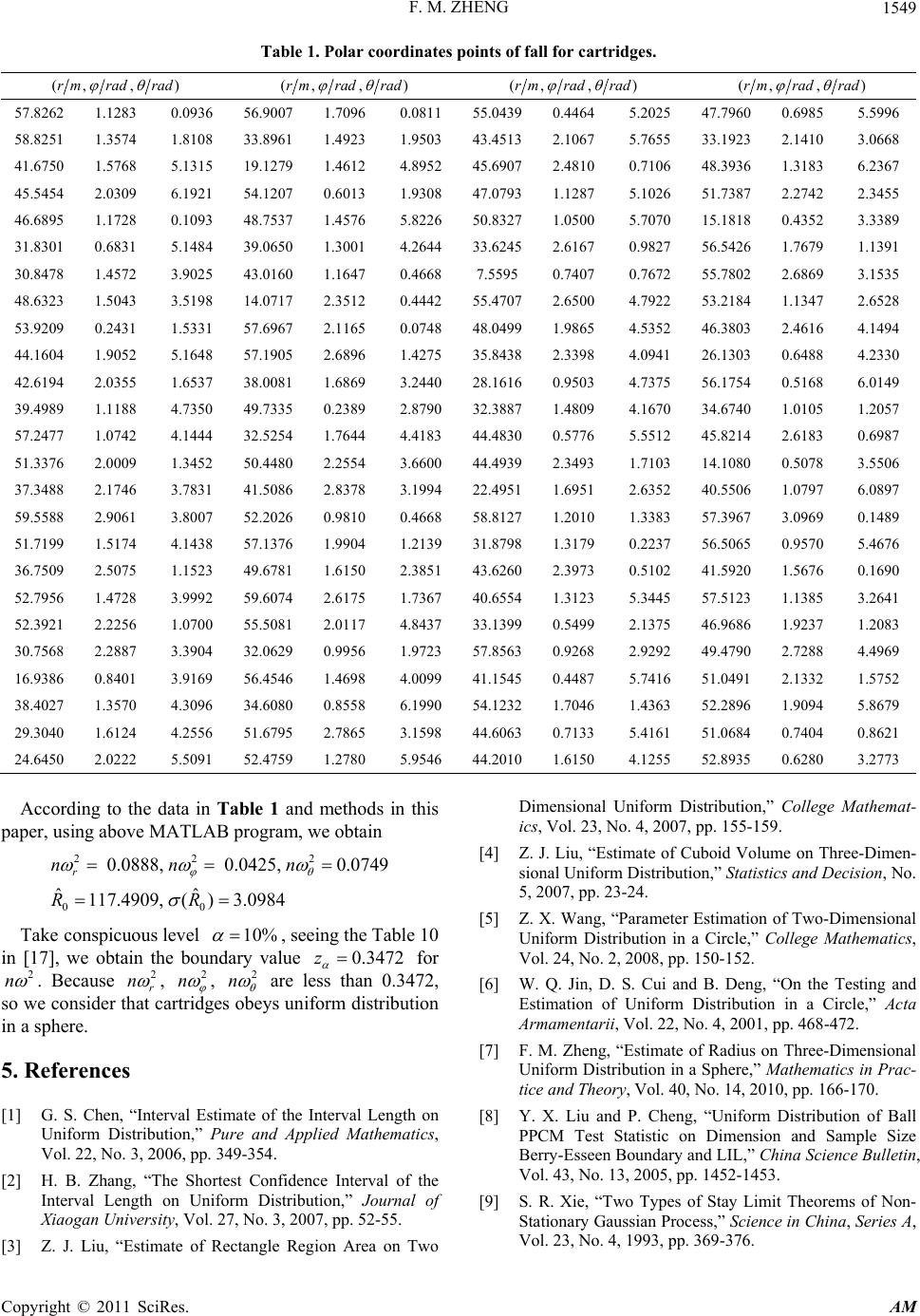

F. M. ZHENG 1549
Table 1. Polar coordinates points of fall for cartridges.
(, ,rm rad rad  )(,, )rm rad rad  (,, )rm rad rad  (, ,rm rad rad  )
57.8262 1.1283 0.9007 1.7096 0.04390.4464 5.7960 0.6985 5.0936 56.0811 55.2025 47.5996
58.8251 1.3574 1.8961 1.4923 1.45132.1067 5.1923 2.1410 3.8108 33.9503 43.7655 33.0668
41.6750 1.5768 5.1315 19.1279 1.4612 4.8952 45.69072.4810 0.7106 48.3936 1.3183 6.2367
45.5454 2.0309 6.1921 54.1207 0.6013 1.9308 47.07931.1287 5.1026 51.7387 2.2742 2.3455
46.6895 1.1728 0.1093 48.7537 1.4576 5.8226 50.83271.0500 5.7070 15.1818 0.4352 3.3389
31.8301 0.6831 5.1484 39.0650 1.3001 4.2644 33.62452.6167 0.9827 56.5426 1.7679 1.1391
30.8478
48.6323 1.
1.4572 3.
5043
9025
3.5198 14.
43.0160
0717 2.
1.1647 0.
3512
4668 7.
0.4442 55.
5595 0.
4707
7407 0.
2.6500
7672
4.7922 53.
55.7802
2184 1.
2.6869
1347
3.1535
2.6528
53.9209 0.2431 1.5331 57.6967 2.1165 0.0748 48.04991.9865 4.5352 46.3803 2.4616 4.1494
44.1604 1.9052 5.1648 57.1905 2.6896 1.4275 35.84382.3398 4.0941 26.1303 0.6488 4.2330
42.6194 2.0355 1.6537 38.0081 1.6869 3.2440 28.16160.9503 4.7375 56.1754 0.5168 6.0149
39.4989 1.
57.2477 1.
1188
0742
4.7350 49.
4.1444 32.
7335 0.
5254 1.
2389
7644
2.8790 32.
4.4183 44.
3887
4830
1.4809
0.5776
4.1670 34.
5.5512 45.
6740 1.
8214 2.
0105
6183
1.2057
0.6987
51.3376 2.0009 1.3452 50.4480 2.2554 3.6600 44.49392.3493 1.7103 14.1080 0.5078 3.5506
37.3488 2.1746 3.7831 41.5086 2.8378 3.1994 22.49511.6951 2.6352 40.5506 1.0797 6.0897
59.5588 2.9061 3.8007 52.2026 0.9810 0.4668 58.81271.2010 1.3383 57.3967 3.0969 0.1489
51.7199 1.
36.7509 2.
5174
5075
4.1438 57.
1.1523 49.
1376 1.
6781 1.
9904
6150
1.2139 31.
2.3851 43.
8798
6260
1.3179
2.3973
0.2237 56.
0.5102 41.
5065 0.
5920 1.
9570
5676
5.4676
0.1690
52.7956 1.4728 3.9992 59.6074 2.6175 1.7367 40.65541.3123 5.3445 57.5123 1.1385 3.2641
52.3921 2.2256 1.0700 55.5081 2.0117 4.8437 33.13990.5499 2.1375 46.9686 1.9237 1.2083
30.7568 2.2887 3.3904 32.0629 0.9956 1.9723 57.85630.9268 2.9292 49.4790 2.7288 4.4969
16.9386 0.
38.4027 1.
8401
3570
3.9169 56.
4.3096 34.
4546 1.
6080 0.
4698
8558
4.0099 41.
6.1990 54.
1545
1232
0.4487
1.7046
5.7416 51.
1.4363 52.
0491 2.
2896 1.
1332
9094
1.5752
5.8679
29.3040 1.6124 4.2556 51.6795 2.7865 3.1598 44.60630.7133 5.4161 51.0684 0.7404 0.8621
24.6450 2.0222 5.5091 52.4759 1.2780 5.9546 44.20101.6150 4.1255 52.8935 0.6280 3.2773
in d s i
aper, using above MATLAB program, we obtain
Take conspicuous level
Accordg to the data in Table 1 anmethodn this
p
222
0.0888, 0.0425,0.0749
r
nnn

 
00
ˆˆ
117.4909, ()3.0984RR  
10%


, seeing the Table
in [17], we obtain the boue
10
ndary valu0.3472z

2
for
n

. Because 2
r
n

, 2 n


, 2 n


are less than 0.3472,
so we consider that cartridges obeys uniftion
sphere.
5. Referen
orm distribu
in a
ces
nterval Estimate of the Interval Length on
Uniform Distribution,” Pure and Applied Mathematics
bution,” Journal
im UDi,” Mt-
ics, Vol. 23, No. 4, 2007, pp. 155-159.
n-
i and B. Deng, “On the Testing and
ensional
of Ball
D ensionalniform stributionCollege athema
[1] G. S. Chen, “I
Uni
, P
Vol. 22, No. 3, 2006, pp. 349-354.
[2] H. B. Zhang, “The Shortest Confidence Interval of the
Interval Length on Uniform Distriof
Xiaogan University, Vol. 27, No. 3, 2007, pp. 52-55.
[3] Z. J. Liu, “Estimate of Rectangle Region Area on Two
[4] Z. J. Liu, “Estimate of Cuboid Volume on Three-Dime
sional Uniform Distribution,” Statistics and Decision, No.
5, 2007, pp. 23-24.
[5] Z. X. Wang, “Parameter Estimation of Two-Dimensional
Uniform Distribution in a Circle,” College Mathematics,
Vol. 24, No. 2, 2008, pp. 150-152.
[6] W. Q. Jin, D. S. Cu
Estimation of Uniform Distribution in a Circle,” Acta
Armamentarii, Vol. 22, No. 4, 2001, pp. 468-472.
[7] F. M. Zheng, “Estimate of Radius on Three-Dim
form Distribution in a Sphere,” Mathematics in Prac-
tice and Theory, Vol. 40, No. 14, 2010, pp. 166-170.
[8] Y. X. Liu and P. Cheng, “Uniform Distribution
PCM Test Statistic on Dimension and Sample Size
Berry-Esseen Boundary and LIL,” China Science Bulletin,
Vol. 43, No. 13, 2005, pp. 1452-1453.
[9] S. R. Xie, “Two Types of Stay Limit Theorems of Non-
Stationary Gaussian Process,” Science in China, Series A,
Vol. 23, No. 4, 1993, pp. 369-376.

F. M. ZHENG 1550
r the Number and [10] Z. S. Hu and C. Su, “Limit Theorems fo
Sum of Near-Maxima for Medium Tails,” Statistics &
Probability Letters, Vol. 63, No. 3, 2003, pp. 229-237.
doi:10.1016/S0167-7152(03)00085-3
[11] Y. Qi, “Limit Distributions for Products of Sums,” Statis-
tics & Probability Letters, Vol. 62, No. 1, 2007, pp. 93-
100. doi:10.1016/S0167-7152(02)00438-8
[12] G. Rempala and J. Wesolowski, “Asymptotics for Prod-
tical Anal
ucts of Sums and U-Statistics,” Electronic Communica-
tions in Probability, Vol. 7, No. 7, 2002, pp. 47-54.
[13] K. T. Fang, J. Q. Fan, H. Jin, et al., “Statisysis
of Directional Date,” Journal of Application of Statistics
and Management, Vol. 9, No. 2, 1990, pp. 59-65.
[14] M. D. Troutt, W. K. Pang and S. H. Hou, “Vertical Den-
sity Representation and Its Applications,” World Scien-
tific Publishing Co. Pte. Ltd, Singapore, 2004.
doi:10.1142/9789812562616
[15] Z. S. Wei, “Probability Theory and Mathematic
tics,” Higher Education Press,
al Statis-
Beijing, 1983.
ility Theory
[16] S. M. Berman, “Extreme Sojourns of a Gaussian Process
with a Point of Maximum Variance,” Probab
and Related Fields, Vol. 74, 1987, pp. 113-124.
doi:10.1007/BF01845642
[17] C. P. Pan and Z. J. Han, “Probability and Statistic o
Weapon Test,” National D
f
efence Industry Press, Beijing,
sidual Quadratic Sums in the Dispersion Equation
1979.
[18] N. I. Sidnyaev and K. S. Andreytseva, “Independence of
the Re
with Noncentral χ2-Distribution,” Applied Mathematics,
Vol. 2, No. 2, 2011, pp. 1303-1308.