Applied Mathematics, 2011, 2, 1515-1521
doi:10.4236/am.2011.212214 Published Online December 2011 (http://www.SciRP.org/journal/am)
On Solutions of Generalized Bacterial Chemotaxis
Model in a Semi-Solid Medium
Ahmed M. A. El-Sayed1, Saad Z. Rida2, Anas A. M. Arafa2
1Department of Mathematics, Faculty of Science, Alexandria University, Alexandria, Egypt
2Department of Mathematics, Faculty of Science, South Valley University, Qena, Egypt
Received July 4, 2011; revised October 22, 2011; accepted October 31, 2011
Abstract
In this paper, the Adomian’s decomposition method has been developed to yield approximate solution of
bacterial chemotaxis model of fractional order in a semi-solid medium. The fractional derivatives are de-
scribed in the Caputo sense. The method introduces a promising tool for solving many linear and nonlinear
fractional differential equations.
Keywords: Decomposition Method, Bacterial Chemotaxis, Semi-Solid Medium, Fractional Calculus
1. Introduction and Preliminaries
This paper deals with numerical solutions of bacterial
chemotaxis model of fractional order in a semi-solid me-
dium. We are primarily interested in describing the be-
haviour of the generalized biological mechanisms that
govern the bacterial pattern formation processes in the
experiments of Budrene and Berg [1] for populations of
E. coli. The model for the semi-solid medium experiment
with E. coli is considered. The key players in this paper
seem to be the bacteria, the chemoattractant (aspartate)
and the stimulant (succinate) so the three variables is
considered: the cell density u, the chemoattractant con-
centration v, and the stimulant con centration w. The bac-
teria diffuse, move chemotactically up gradients of the
chemoattractant, proliferate and become non -motile. The
non-motile cells can be thought of as dead, for the pur-
pose of the model. The chemoattractant diffuses, and is
produced and ingested by the bacteria while the stimu-
lant diffuses and is consumed by the bacteria. The model
consisting of three conservation equations is:
Rate of change of
cell density, u = Diffusion of u +Chemotaxis of u to v + Proliferation
(growth and
death) of u
Rate of change of
chemoattratant
concentration, v = Diffusion of
v +Production of v by u – Uptake of v by u
Rate of change of
stimulant
concentration, w = Diffusion of
w –Uptake of w by u
In recent years, fractional calculus starts to attract
much more attention of physicists and mathematicians. It
was found that various; especially interdisciplinary ap-
plications can be elegantly modeled with the help of the
fractional derivatives. Other authors have demonstrated
applications of fractional derivatives in the areas of elec-
trochemical processes [2,3], dielectric polarization [4],
colored noise [5], viscoelastic materials [6-9] and chaos
[10]. Mainardi [11] and Rossikhin and Shitikova [12]
presented survey of the application of fractional deriva-
tives, in general to solid mechanics, and in particular to
modeling of viscoelastic damping. Magin [13-15] pre-
sented a three part critical review of applications of frac-
tional calculus in bioengineering. Applications of frac-
tional derivatives in other fields and related mathematical
tools and techniques could be found in [16-18]. Rida et
al. presented a new solutions of some bio-mathematical
models of fractional order [19-24].
In this paper, we implemented the Adomian’s decom-
position method (ADM) [25,26] to the generalized bacte-
rial pattern formation models in a semi-solid medium:
2
214
3
22
29
2
257
2
6
2
282
9
,
()
u
v
w
kuk w uDuvku u
tkvkw
vu
Dvkw kuv
tku
ww
Dwku
tkw






 

 


 




(1.1)

A. M. A. EL-SAYED ET AL. 1516
where 01

,
concentration
respectively. There
alues (,uv
del.
,uv
of the chem
are
,wa
and are the cell density, the
actant and of the stimulant
three diffusion coefficients, three
initial v and nine parameters
the mo
Subject to initial conditions:
and
where and are the cell density, the concentratio
oattractant and of
stems of Ein
the first time derivative term by a fractional
de
w
oattr
0)t tk in
n
0
(,0) ()uu, 0 (,0) ()vv 0 (,0) ()ww 
,uv
hem w
al sy
of the cthe stimulant respectively.
There are three diffusion co efficients, three initial values
(,, at0)uvw t and nine parameters k in the model.
The fractionquations (1.1) are obtaed
by replacing
rivative of order 0

. The Derivatives are under-
stood in the Caputo sense. The g
sion contains a parameter desche order of the
al tiv
eneral response expres-
ribing t
fractionderivae that can be varied to obtain various
responses.
In the case of 1

, the fractional system equations
ndard system of partiadifferential equreduce to the stal a-
tio
ntial
des in any symbolic languages. The method
pr in the
, the
fu
tion of the method is extended for fractional differential
equations [30-33].
n of differentiation to fractional orders e.g. Rie-
m
ions for fractional order differential
eq
me form as for integer
rder differential equations. derivative of
ns. The Adomian’s decomposition method will be
applied for computing solutions to the systems of frac-
tional partial differeequations considered in this
paper. This method has been used to obtain approximate
solutions of a large class of linear or nonlinear differen-
tial equations. It is also quite straightforward to write
computer co
ovides solutions form of power series with easily
computed terms. It has many advantages over the classi-
cal techniques mainly; it provides efficient numerical
solutions with high accuracy, minimal calculations.
The reason of using fractional order differential equa-
tions (FOD) is that FOD are naturally related to systems
with memory which exists in most biological systems.
Also they are closely related to fractals which are abun-
dant in biological systems. The results derived of the
fractional system (1.1) are of a more general nature. Re-
spectively, solutions to the fractional reaction-diffusion
equations spread at a faster rate than the classical diffu-
sion equation, and may exhibit asymmetry. However
ndament al so l ut i on s o f t h ese equations still exhibit use-
ful scaling p roperties that make them attractive for appli-
cations.
Cherruault [27] proposed a new definition of the me-
thod and he then insisted that it would become possible
to prove the convergence of the decomposition method.
Cherruault and Adomian [28] proposed a new conver-
gence series. A new approach of the decomposition me-
thod was obtained in a more natural way than was given
in the classical presentation [29]. Recently, the applica-
There are several approaches to the generalization of
the notio
ann-Liouville, GruÖnwald-Letnikow, Caputo and Ge-
neralized Functions approach [34]. Riemann-Liouville
fractional derivative is mostly used by mathematicians
but this approach is not suitable for real world physical
problems since it requires the definition of fractional
order initial conditions, which have no physically mean-
ingful explanation yet. Caputo introduced an alternative
definition, which has the advantage of defining integer
order initial condit
uations [34]. Unlike the Riemann-Liouville approach,
which derives its definition from repeated integration,
the GruÖnwald-Letnikow formulation approaches the
problem from the derivative side. This approach is most-
ly used in numerical algorithms.
2. Fractional Calculus
Here, we mention the basic definitions of the Caputo
fractional-order integration and differentiation, which are
used in the up coming paper and play the most important
role in the theory of differential and integral equation of
fractional order.
The main advantages of Caputo’s approach are the ini-
tial conditions for fractional differential equations with
Caputo derivatives take on the sa
oDefinition 2.1 The fractional()
f
x in
e Caputo sense is defined as [34]: th
1()
0
() ()
1() ()d
()
mm
x
mm
DfxIDfx
x
tftt
m







 
for 1,mm


 ,mN

0x.
For the Caputo derivative we have 0DC


, C is
constant
( 1)
1)
n
n


0,
(1) ,(
(1)
n
n
Dt nt
n














Definition 2.2 For to be the smallest integer that
exceeds


m

, the Caputo fractional derivatives of order
0

 is defined as [34]:
1
0
(,)
(,)
1(
ux
uxt t




,)
()d,for 1
()
(,)
,for
tm
m
m
m
m
D
ux
tm m
m
uxt mN
t







t






 















A. M. A. EL-SAYED ET AL.1517
3.
To givolution of nonlinear fractional-
order differential equations by means of the ADM, we
write the systems in the form
(3.1)
e fractional operators,
nd nonlinear operators.
Analysis of the Method
e the approximate s
1
2
1112 1
2212 2
12
(,)(, ,,)(,)
(,)(, ,,)(,)
(,)(, ,,)(,)
m
m
m
mm mm
Dut Nuuuft
Dut Nuuuft
Dut Nuuuft



 
 
 




where (1,2,,)
i
Di m

 are th
a12
Applying the inverse operators 12 ,,,
,, m NN N are
M
III
 
 to
the systems (3.1)

1




(3.2)
(3.3)
d suggests that
are decomposed by an infinite se-
ries of com
and the nonlinear operators are defined by the infinite
series of the so called Adomian polynomials
n
w


2
11121
22122
12
(,)(, ,,)(,)
(,)(, ,,)(,)
(,)(, ,,)(,)
M
m
m
mmmm
utINuuuft
utINuuu ft
utINuuuft


 
 
 




Subject to the initial conditions
)(),(1,2, ,)
i
gi m  (,0
i
u
The Adomian decomposition metho the
linear terms (,ut)
i
ponents
,
0
(,)(,),(1,2, ,)
iin
n
utu tim


 
 (3.4)
,
0
ii
n
NA


 (3.5)
here ,(,)
in
ut; 0n are the components of (,)
i
ut

,
that will be elegantly determined, and ,in
A
; 0n are
Adomian’s polynomials that can be generated
forms of non linearity [35]. Substituting (3.4) and (3.5)
into (3.2) gives


ed into a set of recursive relations given
by
for all
1
1,11, 1
00
(,) ()(,)
nn
nn
utg IAft




 



2
2, 2
00
(,
) ()
n
nn
ut
g I




  

 2,2 (,)
n
Aft
 

(3.6)
,,
00
(, ) ()(,)
m
mn mmn m
nm
ut g IAft




  




Following adomian analysis, the nonlinear system
(3.1) is transform

,0
,1 ,
(,) ()
(,)(,) 0,
ii
inin i
utg
utIAftn






(3.7)
where (1,2,,)im

.
It is an essential feature of the decomposition m
that the zeroth components are defined always
by all terms that arise from integrat-
ing the inhomogeneous termaining pairs
can be easily determined in a parallel man-
omponents of , the solutions of the
me of a power series
expansion upon using (3.4). es obtain
any cases to closed form solution
problemthe approximants can be
us
qualitative
work, s
ethod
,0 (,) i
ut
initial data and from
s. The rem
(,)
i
ut
diately in the form
The seri
give a
n term
,in
r. Additional pairs for the decomposition series nor-
mally account for higher accuracy. Have been deter-
min
(, 1)un
ne
ed the c
system follow im
summed up in m
crete
ed can be
for cons,
ed for numerical purposes. Comparing the scheme
presented above with existing techniques such as charac-
teristics method and Riemann invariants, it is clear that
the decomposition method introduces a fundamental
difference in approach, because no assump-
tions are made. The approach is straightforward and the
rapid convergence is guaranteed. To give a clear over-
view of the content of this everal illustrative ex-
amples have been selected to demonstrate the efficiency
of the method.
4. Applications and Numerical Results
In order to illustrate the advantages and the accuracy of
the ADM, we consider time-fractional chemotaxis model
of bacteria colonies in a semi-solid medium (1.1) in one
dimensional in the form:
2
14
3
22
29
()
uxx
xx
Du DLu
kuk w
LLvkuu
kv kw


 
2
2
u
w

52
6
vx
x
Dv DLv kw
ku
82
9
wx x
Dw DLw ku
kw



 


 
(4.2)




Subject to the initial conditions
ux 0 (,0)n
2
(,0)
x
vx e




0
(,0)wx s
where 00 ,,,ns


Operating with
are constants.
I

in both sides of system (4.2) we
find

A. M. A. EL-SAYED ET AL. 1518
2
14
3
2
29
2
52
6
2
82
9
(,) (,0)
()
(,) (,0)
(,) (,0)
uxx xx
vxx
wxx
uxt ux
kuk w
2
I
DL uLLvkuu
kv kw
u
vxtvxIDL vkw
ku
w
wxtwxIDL wku
kw





 
 
 



 


 





 






(4.3)
The ADM assumes a series solution for
and given by:
Substituting the decomposition series (4.4) into (4.3)
yields
0 n
(,),(,)uxtvxt
(,)wxt
0
0
(,)( )
(
(,) (,)
n
n
n
n
uxtuxt
vx
wxtw xt








0
,) (,)
n
n
tvxt

 (4.4)
,

0
1343
000
(,) (,0)
(,)
n
n
uxxnxnnn
nnn
uxt ux
I
DLu xtkLAkkBkC















0n

 

0
n
n



Identifying the zeros components, and
by and
can be det
recurrence relation:

(4.6

(4.7)
where
5
(,) (,0)(,)
nvxxn
vxtvxI DLvxtkD



 


00nn 

n
8
00
(,) (,0)(,)
nwxxn
nn
wxtwxI DLwxt kB




 



00
(,), (,)uxtvxt
(x
0(,)wxt
component 00
(,0), (,0)ux vx
s where 0n0
w,0) the remaining
ermined by using
00
(,) (,0)
0
uxt ux
u
n


11 343
(,) (),
nuxxnxnnn
x
tIDLukLAkkBkC



(4.5)
00
15
(,) (,0)
(,) (),0
nvxxnn
vxt vx
vxtIDLvkD n



 )
00
18
(,) (,0)
(,)(), 0
nwxxnn
wxt wx
wxtIDLwkBn




n
A
, n B,
als calculated for all fo
n
C
100 0
00
220
2
0
11201 2
0
)
v
Au kuv v


20 2
,
()
1
(
x
kuv v
Au
xk v kv
xkvx k




 
(4.8)
2
0
B00
2
90
2
10 9001
122
90 90
2
()
uw
kw
uw kuww
Bkw kw



(4.9)
1
u
(4.10)
and
2
00
10
2
Cu
Cu


2
00
02
60
2
106 001
122
6060
()ku ku


Using Equations (4.5)-(4.11), we can calculate
2
wu
Dku
wukwuu
D

some
of the terms of the decomposition series (4.4) as:
(4.11)
0(,) ()uxtfx
11
(,)() (1)
t
uxt fx



2
22
(,)() (2 1)
t
uxtfx



0(,) ()vxt gx
11
(,)() (1)
t
vxt gx



2
t

22
(,)() (2 1) vxtgx


and
0(,) ()wxt hx
11
(,)() (1)
t
wxt hx



2
22
(,)() (2 1) wxt hx
 
where:
t


0
()
f
xn
2
(2) 2
1134
2
29
() u
gfh
3
f
xDfkfkkkf
xk gkh

 
 
(2)
211121 2
22
291
1
343 1
222
99
() ()
22
()
u
gg
fxDfkfkfg
xkgx kg
kfhh fh
kkk f f
khkh


 

 







,
, and are the Adomian’s polyno-
mi s of nonlinearity according
to specific algorithms constructed by Adomian as:
n
D
rm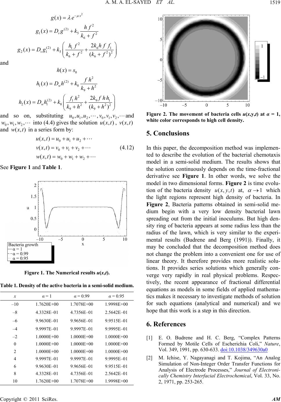

A. M. A. EL-SAYED ET AL.1519
2
()
x
gx e




2
(2)
15
2
6
() v
hf
gx Dgkkf 

2
(2) 61 1
215
22
66
2
() ()
v
khff hf
gxDgk kf kf

 




2
and
0
()hx s
2
(2)
18
2
9
() w
f
h
hx Dhkkh 

2
(2) 91
1
218
22
99
2
() ()
w
kfhh fh
hxDhk kh kh

 




2
and so on, substituting 012 ,,,uuu,012 ,,,vvv


(,)uxt, (,vx
and
into (4.4) gives the solution
in a series form
(4.12)
See Figure 1 and Table 1.
012
,,,www
and (,)wxt
)
t
by:
012
012
012
(,)
(,)
(,)
uxtuu u
vxtvv v
wxtww w






Figure 1. The Numericau
ity of the active bacteria in a sem.
α = 1 α
l results (x,t).
Table 1. Densi-solid medium
x = 0.99 α = 0.95
–10 1.7620E+00 1.7078E+00 1.9998E+00
–8 4.3328E–01 4.7356E–01
–6 9.9630E–01 9.9656E–01 9.9515E–01
9.9997E–01 9.9995E–01
–2 1.0000E+00 1.0000E+00 1.0000E+00
0 1.0000E+00 1.0000E+00 1.0000E+00
2 1.0000E+00 1.0000E+00 1.0000E+00
4 9.9997E–01 9.9997E–01 9.9995E–01
6 9.9630E–01 9.9656E–01 9.9515E–01
8 4.3328E–01 4.7356E–01 2.5642E–01
10 1.7620E+00 1.7078E+00 1.9998E+00
2.5642E–01
–4 9.9997E–01
Figure 2. The movement of bacteria cells u(x,y,t)at α = 1,
5. Coclusion
In thaper, tosit wa-
ted tscribeion eriais
mode a seediuultat
the solution codep timl
derivative see In s, we
mode two d for 2 i
tion ofthe bac
white color corresponds to high cell density.
ns
is phe decompion methods implemen
o de the evolutof the bactl chemotax
l inmi-solid mm. The ress shows th
ntinuously ends on thee-fractiona
Figure 1. other worde solve th
l inimensionalms. Figure s time evolu-
teria density(,,) at, uxyt1


of bacteria.
which
the light regions n
Figure 2, Bacns obtaine seme-
diumegin w lo ban
spreading out itia. B-
sity ring of bacteria appears at some radius less than the
radius of the lawn, which is very similar to the experi-
mental results (Budrene and Berg (1991)). Finally, it
may be concluded that the decomposition method does
not change the problem into a convenient one for use of
linear theory. It therefore provides more realistic solu-
tions. It provides series solutions which generally con-
verge very rapidly in real physical problems. Respec-
tively, the recent appearance of fractional differential
equations as models in some fields of applied mathema-
tics makes it necessary to investigate methods of solution
for such equations (analytical and numerical) and we
hope that this work is a step in this direction.
and H. C. Berg, “Complex Patterns
tile Cells of Escherichia Coli,” Nature,
Vol. 349, 1991, pp. 630-633. doi:10.1038/349630a0
represent high density I
teria patter
ith a veryd in w densityi-solid m cterial law bfrom the inl inoculumsut high den
6. References
[1] E. O. Budrene
Formed by Mo
2, 1971, pp. 253-265.
[2] M. Ichise, Y. Nagayanagi and T. Kojima, “An Analog
Simulation of Non-Integer Order Transfer Functions for
Analysis of Electrode Processes,” Journal of Electroni-
cally Chemistry Interfacial Electrochemical, Vol. 33, No.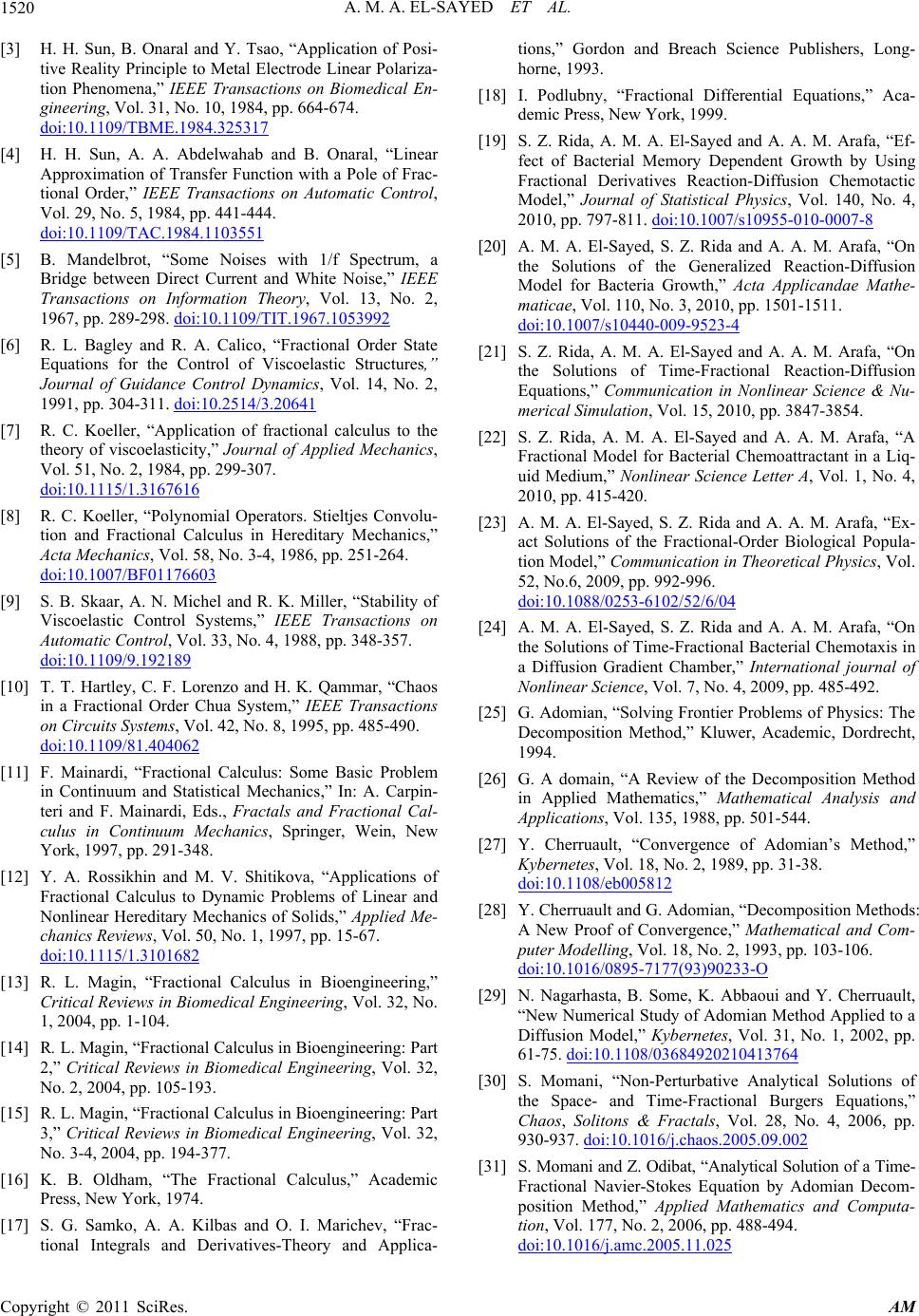

A. M. A. EL-SAYED ET AL. 1520
[3] H. H. Sun, B. Onaral and Y. Tsao, “Application of Posi-
tive Reality Principle to Metal Electrode Linear Polariza-
tion Phenomena,” IEEE Transactions on Biomedical En-
gineering, Vol. 31, No. 10, 1984, pp. 664-674.
doi:10.1109/TBME.1984.325317
[4] H. H. Sun, A. A. Abdelwahab and B. Onaral, “Linear
Approximation of Transfer Function with a Pole of Frac-
tional Order,” IEEE Transactions on Automatic Control,
Vol. 29, No. 5, 1984, pp. 441-444.
doi:10.1109/TAC.1984.1103551
[5] B. Mandelbrot, “Some Noises with 1/f Spectrum, a
Bridge between Direct Current and White Noise,” IEEE
Transactions on Information Theory, Vol. 13, No. 2,
1967, pp. 289-298. doi:10.1109/TIT.1967.1053992
[6] R. L. Bagley and R. A. Calico, “Fractional Order State
Equations for the Control of Viscoelastic Structures,”
Journal of Guidance Control Dynamics, Vol. 14, No. 2,
1991, pp. 304-311. doi:10.2514/3.20641
[7] R. C. Koeller, “Application of fractional calculus to the
theory of viscoelasticity,” Journal of Applied Mechanics,
Vol. 51, No. 2, 1984, pp. 299-307.
doi:10.1115/1.3167616
[8] R. C. Koeller, “Poly
tion and Fractnomial Operators. Stieltjes Convolu- ional Calculus in Hereditary Mechanics,
Acta Mechanics, Vol. 58, No. 3-4, 1986, pp. 251-264. ”
doi:10.1007/BF01176603
[9] S. B. Skaar, A. N. Michel and R. K. Miller, “Stability of
Viscoelastic Control Systems,” IEEE Transactions on
Automatic Control, Vol. 33, No. 4, 1988, pp. 348-357.
doi:10.1109/9.192189
[10] T. T. Hartley, C. F. Lorenzo and H. K. Qammar, “Chaos
in a Fractional Order Chua System,” IEEE Transactions
on Circuits Systems, Vol. 42, No. 8, 1995, pp. 485-490.
doi:10.1109/81.404062
[11] F. Mainardi, “Fractional Calculus: Some Basic Problem
in Continuum and Statistical Mechanics,” In: A. Carpin-
teri and F. Mainardi, Eds., Fractals and Fractio
culus in Continuum Mechanics, nal Cal- Springer, Wein, New
Solids,” Applied Me-
. 15-67.
York, 1997, pp. 291-348.
[12] Y. A. Rossikhin and M. V. Shitikova, “Applications of
Fractional Calculus to Dynamic Problems of Linear and
Nonlinear Hereditary Mechanics of
chanics Reviews, Vol. 50, No. 1, 1997, pp
doi:10.1115/1.3101682
[13] R. L. Magin, “Fractional Calculus in Bioengineering,”
Critical Reviews in Biomedical Engineering , Vol. 32, No.
1, 2004, pp. 1-104.
[14] R. L. Magin, “Fractional Calculus in Bioengineering: Part
2,” Critical Reviews in Biomedical Engineering , Vol. 32,
No. 2, 2004, pp. 105-193.
[15] R. L. Magin, “Fractional Calculus in Bioengineering: Part
alculus,” Academic
-
ory Dependent Growth by Using
3,” Critical Reviews in Biomedical Engineering , Vol. 32,
No. 3-4, 2004, pp. 194-377.
[16] K. B. Oldham, “The Fractional C
Press, New York, 1974.
[17] S. G. Samko, A. A. Kilbas and O. I. Marichev, “Frac-
tional Integrals and Derivatives-Theory and Applica-
tions,” Gordon and Breach Science Publishers, Long
horne, 1993.
[18] I. Podlubny, “Fractional Differential Equations,” Aca-
demic Press, New York, 1999.
[19] S. Z. Rida, A. M. A. El-Sayed and A. A. M. Arafa, “Ef-
fect of Bacterial Mem
Fractional Derivatives Reaction-Diffusion Chemotactic
Model,” Journal of Statistical Physics, Vol. 140, No. 4,
2010, pp. 797-811. doi:10.1007/s10955-010-0007-8
[20] A. M. A. El-Sayed, S. Z. Rida and A. A. M. Arafa, “On
the Solutions of the Generalized Reaction-Diffusion
Model for Bacteria Growth,” Acta Applicandae Mathe-
maticae, Vol. 110, No. 3, 2010, pp. 1501-1511.
doi:10.1007/s10440-009-9523-4
[21] S. Z. Rida, A. M. A. El-Sayed and A. A. M. Arafa, “On
a, “A
erial Chemoattractant in a Liq-
S. Z. Rida and A. A. M. Arafa, “Ex-
6.
the Solutions of Time-Fractional Reaction-Diffusion
Equations,” Communication in Nonlinear Science & Nu-
merical Simulation, Vol. 15, 2010, pp. 3847-3854.
[22] S. Z. Rida, A. M. A. El-Sayed and A. A. M. Araf
Fractional Model for Bact
uid Medium,” Nonlinear Science Letter A, Vol. 1, No. 4,
2010, pp. 415-420.
[23] A. M. A. El-Sayed,
act Solutions of the Fractional-Order Biological Popula-
tion Model,” Communication in Theoretical Physics, Vol.
52, No.6, 2009, pp. 992-99
doi:10.1088/0253-6102/52/6/04
[24] A. M. A. El-Sayed, S. Z. Rida and A. A. M. Arafa, “On
the Solutions of Time-Fractional Bacterial Chemotaxis in
“A Review of the Decomposition Method
a Diffusion Gradient Chamber,” International journal of
Nonlinear Science, Vol. 7, No. 4, 2009, pp. 485-492.
[25] G. Adomian, “Solving Frontier Problems of Physics: The
Decomposition Method,” Kluwer, Academic, Dordrecht,
1994.
[26] G. A domain,
in Applied Mathematics,” Mathematical Analysis and
Applications, Vol. 135, 1988, pp. 501-544.
[27] Y. Cherruault, “Convergence of Adomian’s Method,”
Kybernetes, Vol. 18, No. 2, 1989, pp. 31-38.
doi:10.1108/eb005812
[28] Y. Cherruault and G. Adomian, “Decomposition Methods:
A New Proof of Convergence,” Mathematical and Com-
puter Modelling, Vol. 18, No. 2, 1993, pp. 103-106.
doi:10.1016/0895-7177(93)90233-O
[29] N. Nagarhasta, B. Some, K. Abbaoui and Y. Cherruault,
“New Numerical Study of Adomian Method App
Diffusion Model,” Kybernetes, Vlied to a ol. 31, No. 1, 2002, pp.
61-75. doi:10.1108/03684920210413764
[30] S. Momani, “Non-Perturbative Analytical Solutions of
the Space- and Time-Fractional Burgers Equations,”
Chaos, Solitons & Fractals, Vol. 28, No. 4, 2006, pp.
930-937. doi:10.1016/j.chaos.2005.09.002
[31] S. Momani and Z. Odibat, “Analy tical Solution of a Time-
Fractional Navier-Stokes Equation by Adomian Decom-
position Method,” Applied Mathematics and Computa-
tion, Vol. 177, No. 2, 2006, pp. 488-494.
doi:10.1016/j.amc.2005.11.025

A. M. A. EL-SAYED ET AL. 1521
Differential Equations of
ns & Fractals, Vol. 31,
[32] S. Momani and Z. Odibat, “Numerical Comparison of
Methods for Solving Linear
Fractional Order,” Chaos, Solito
[34] I. Podlubny and A. M. A. El-Sayed, “On Two Definition
of Fractional Calculus,” Solvak Academy of Science-
pplied Mathe-
11, No. 1, 2000, pp. 53-
Institute of Experimental Physics, UEF-03-96 ISPN 80-
7099-252-2, 1996.
[35] A. Wazwaz, “A New Algorithm for Calculating Adomian
Polynomials for Nonlinear Operators,” A
matics and Computation, Vol. 1
No. 5, 2007, pp. 1248-1255.
doi:10.1016/j.chaos.2005.10.068
[33] Z. Odibat and S. Momani, “Approximate Solutions for
Boundary Value Problems of Time-Fractional Wave
Equation,” Applied Mathematics and Computation, Vol.
181, No. 1, 2006, pp. 767-774.
doi:10.1016/j.amc.2006.02.004
69. doi:10.1016/S0096-3003(99)00063-6
Note: Parameters Taken as:
0
968
123
1,0.01, 0.1,
3.9(10) ,5(10) ,1.62(10),kk
63
5678 90
666
1,4(10),1 3(10) ,
24(10) ,8.9(10),9(10),100
kkkk ks
DDt
uvw
n
k


 
 

D

 
 
 