Applied Mathematics, 2011, 2, 1507-1514
doi:10.4236/am.2011.212213 Published Online December 2011 (http://www.SciRP.org/journal/am)
Pattern Formation in Tri-Trophic Ratio-Dependent Food
Chain Model
Dawit Melese, Sunita Gakkhar
Department of Mat hematics, Indian Institute of Technology Roorkee, Roorkee, India
Received October 27, 2011; revised November 26, 2011 ; accepted December 5, 2011
Abstract
In this paper, a spatial tri-trophic food chain model with ratio-dependent Michaelis-Menten type functional
response under homogeneous Neumann boundary conditions is studied. Conditions for Hopf and Turing bi-
furcation are derived. Sufficient conditions for the emergence of spatial patterns are obtained. The results of
numerical simulations reveal the formation of labyrinth patterns and the coexistence of spotted and stripe-
like patterns.
Keywords: Reaction-Diffusion Equations, Hopf Bifurcation, Turing Instability, Turing Pattern, Food Chain
1. Introduction
Food chains in the environment are very important sys-
tems in ecological science, applied mathematics, eco-
nomic and engineering science [1]. They have been ap-
plied to management in Aquatic ecosystem for problems
like water quality and lake management [2]. Modeling of
food chain dynamics has challenges in the fields of both
theoretical ecology and applied mathematics. Tri-trophic
food chain models have been studied in both spatially
homogeneous [1-4] and spatially inhomogeneous envi-
ronments [5-10] for the last two decades. Those models
exhibit rich and complex dynamics and nonlinear mathe-
matical behavior, including varying numbers and stabili-
ty of equilibrium states, limit cycles, patterns and chaos.
It is well known that in real life, the resources are not
uniformly distributed in the habitat. The biological spe-
cies move (diffuse) from place to place in search of food
in their habitat and hence interact with each other and
with the environment. This movement (diffusiveness) of
species has an impact on their trophic interactions. Con-
sequently, spatial pattern s evolve.
One can easily observe patterns in both aquatic and
terrestrial populations [10]. A number of recent contribu-
tions have begun to suggest that it is critical to begin to
fully consider the implications of spatial flows on the
dynamics of ecological communities [7]. In the litera-
tures [11,12], the spatial component of ecological inter-
actions (trophic-interactions) is identified as an important
factor in shaping ecological communities. However, there
is lack of recognition about the role of spatial considera-
tions in food chain dynamics [7]. In addition to this, ig-
norance of spatial scales of fo od chains limits our ability
to predict how trophic interactions will vary in different
contexts, across space and time [2]. The dynamics and
stability of the interacting species in relation to spatial
phenomena such as pattern formation has recently be-
come a focus of intensive research in theoretical ecology
[13], chemical and biological systems [14]. The spatial
patterns modify the temporal dynamics at a range of spa-
tial scales, whose effects must be incorporated in tempo-
ral ecological models that do not represent space explic-
itly. In recent decades, stationary patterns induced by
diffusion have been studied extensively, and lots of im-
portant phen o mena have been obs erved.
Spatial patterns of interacting species are ubiquitous in
nature and may occur due to stochastic process, environ-
mental fluctuations or variability, or deterministic proc-
ess, growth and movement of interacting species. The
deterministic process is intrinsic to the interacting spe-
cies and results in population-driven and self-organized
spatial patterns. The formation of population-driven spa-
tial patterns was first pointed out by Alan Turing. Turing,
one of the key scientist of the 20th century, mathemati-
cally showed that a system of coupled reaction-diffusion
equations can give rise to spatial concentration patterns
of a fixed characteristic length from an arbitrary initial
configuration due to diffusion—driven instability or Tur-
ing instability [15].
Reaction-Diffusion systems are capable of qualitati-
vely imitating many biological patterns such as the stri-
pes of a zebra, tiger and snakes or spots of a cheetah and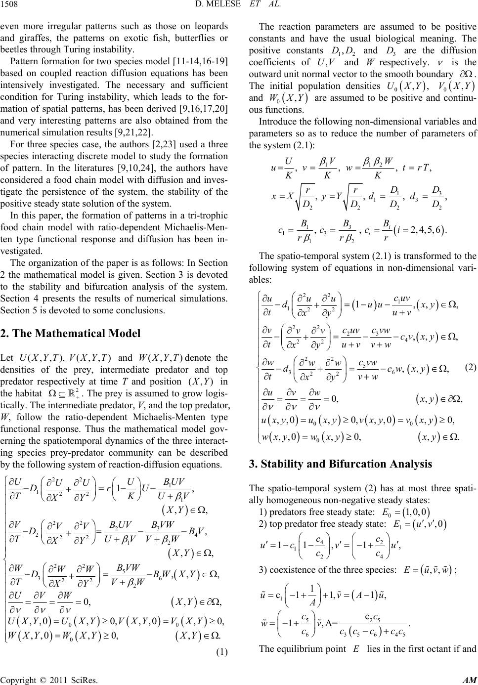

D. MELESE ET AL. 1508
even more irregular patterns such as those on leopards
and giraffes, the patterns on exotic fish, butterflies or
beetles through Turing instab ility.
Pattern formation for two species model [11-14,16-19]
based on coupled reaction diffusion equations has been
intensively investigated. The necessary and sufficient
condition for Turing instability, which leads to the for-
mation of spatial patterns, has been derived [9,16,17,20]
and very interesting patterns are also obtained from the
numerical simulation results [9,21,22].
For three species case, the authors [2,23] used a three
species interacting discrete model to study the formation
of pattern. In the literatures [9,10,24], the authors have
considered a food chain model with diffusion and inves-
tigate the persistence of the system, the stability of the
positive steady state solution of the system.
In this paper, the formation of patterns in a tri-trophic
food chain model with ratio-dependent Michaelis-Men-
ten type functional response and diffusion has been in-
vestigated.
The organization of the paper is as follows: In Section
2 the mathematical model is given. Section 3 is devoted
to the stability and bifurcation analysis of the system.
Section 4 presents the results of numerical simulations.
Section 5 is devoted to some conclusions.
2. The Mathematical Model
Let and denote the
densities of the prey, intermediate predator and top
predator respectively at time T and position
(,,), (,,)U XYTV XYT(,,)WXYT
(,)
X
Y in
the habitat . The prey is assumed to grow logis-
tically. The intermediate predator, V, and the top predator,
W, follow the ratio-dependent Michaelis-Menten type
functional response. Thus the mathematical model gov-
erning the spatiotemporal dynamics of the three interact-
ing species prey-predator community can be described
by the following system of reaction-diffusion equations.
2







22 1
122 1
22 3
2
24
B V
22 12
22 5
36
22 2
0
1,
,,
,
,,
,, ,
0,, ,
,,0, 0,
BUV UU
UU
DrU
TKUV
XY XY
BVW BUV
VVV
D
TUVVW
XY XY
BVW WWW
DBWXY
TVW
XY
UVW XY
UXYU XYV












 







 







 

 



 
0
0
,,0, 0,
,,0, 0,,.
XYV XY
W XYWXYXY
















 


(1)
The reaction parameters are assumed to be posi
co
tive
nstants and have the usual biological meaning. The
positive constants 12 ,DD and 3 D are the diffusion
coefficients of ,UV Wrespectively. and

is the
outward unit norm smooth bounry al vector to theda

.
The initial population densities

0,,UXY


0
VX
and ,Y


0,WXY are assumed to be
ous f
Introduce the f
positive and continu-
unctions. ollowing non-dimensional variables and
parameters so as to reduce the number of parameters of
the system (2.1):
112
3
1
13
222
,, ,,
,,,
VW
2
,
uv wtrT
KK K
D D rr
xXyY dd
DDDD

U 
 


3 1
13
12
,, 2,4,5
i
i
BB B
cc ci
rr r 
  ,6.
The spatio-temporal system (2.1) is transformed to the
following system of equations in non-dimensional vari-
ables:
 




22 1
122
22 3
24
22
22 5
36
22
00
1,,
,, ,
,, ,
0,, ,
,,0, 0,,,0, 0,
,
cuv , uu
duuxy
tuv xy
cvw cuv vvv cv xy
tuvvw xy
cvw www
dcwxy
tvw xy
uvwxy
uxyu xyvxyv xy
wxy


 u

  







 










 



 

 
 
0
,0, 0,,.wxy xy



















(2)
. Stability and Bifurcation Analysis
he spatio-temporal system (2) has at most three spati-
3
T
ally homogeneous non-negative steady states:
1) predators free steady state:

01, 0, 0E
2) top predator free steady state: ,,Eu



10v
42
cc

124
11 ,1,uc vu
cc

  


3) coexistence of the three species:

,,Euvw ;

11
c1 1,1uv
A





,Au


525
63564
c
1,A=
cc
wv
ccccc


 


5
.
c
The equilibrium point lies in the first octant if and
E

D. MELESE ET AL.1509
only if
56 1
,1,0 1
A
ccA c
A

 (3)
From biological point of view the stability of the non-
tri
ity analysis, the spatio-tem-
po
vial steady stateEwhich ensures th e coexistence of the
three species is of interest.
To perform linear stabil
ral system (2) is linearized at the spatially homogene-
ous steady state E for small space and time dependent
fluctuations. For this, set
 
 
 
,,,, ;,,,
,,,, ;,,,
,,,, ;,,.
uxytuu xytuxytu
vxytvv xytvxytv
wxytw wxytwxytw



 


 



Let us assume solutions of the form





0
1
2
,, cos cos,
,,
txy
vx
ytekx ky
wxyt



,,uxyt








 


where

0,1 is the growth rate of perturbation in time t,

,2
ii
  represent the amplitudes,
x
k and
y
k
umber of the solutions. The cos pondi
linearized system has the characteristic equation
are theve n warre ng
20.JkD I
  (4)
Here

13
,1,Ddiagdd, 222
x
y
kk k

 and 33 ()
ij x
Ja

e elementsis the community matrix of the system (2). Th
are obtained as

1
11 11213
22
2
2
26
2
212243
225
2
2
366 6
233132 5336
25
5
1
11,,0,
1,1
,0,1 ,1
c
aca a
AA
Ac c
c
aacc
c AA
ccc c
aaacac
c c5
,
.
c

 



 







 


The characteristic equation corresponding to is

E



3222 2
 (5
21
0
0,bkbk bk   )
with
3
,

22
21122331
((1 )),bka aakdd 



2
111331122223332232112
213223 11133
413 13
1(1)
()
bkaa aaaaaaaa
kddada da
kd ddd





 

2
0113322113223122133
221 12112232233322311133
46
133223111313
().
bkaaaaaa aaa
kaaaadaaaadaa
kdaaddadkdd
 
 

The reaction-diffusion systems have led to the charac-
terization of two basic types of symmetry-breaking bi-
furcations—Hopf and Turing bifurcation, responsible for
the emergence of spatio-temporal patterns. See, for de
tails, references [15,16,23,24]. -
According to Routh-Hurwitz criteria




Re 0k 

if and only if




22222
02120
0, 0,0bk bk bkbkbk  (6)
Contradiction of any one of the above c-
plies the existence of an eigenvalue withl
part, hence, in
onditions im
positive rea
stability. Turing instability (or diffusion
driven instability) occurs if the homogeneous steady
is stable in the absence of diffusion )
state
E 2 (0k

but
driven unstable by diffusion 2
(0)k. Thus we need
two conditions which must hold simultaneously. First,
the spatially uniform steady state must be stable to small
perturbation, that is, all

2
k  in Equation (5) have




20 0k
 Re

, and second, only patte cer-
tain spatial extent, that is, patterns within a definite range
of wave length k, can begin to grow, with
rns of a




2
Re0 0k 

.
It is clear that the homous steady state E is
lly stable if and only if
ogene
locally asymptotica


000,b


200b and




12 0
00 00bb b. But it will be
driven unstable by diffusion if any of the
Equation (3.4) fail to it ca
conditions in
easily hold. However,n be
seen that diffusion driven instability cannot occur by
contradicting


2
20bk . Hence, we have tor
which reverse the other two condi-
tions in Equation (3.4). The expressions for
look fo
conditions sign of the


2
0
bk and






22 2
12 0
bk bkbk are both cubic functions of 2 k
of the form:


2642
321030
;0,0.FkFkFkFk FFF

 
(7)
The coefficients


0, 1,2,3Fi are given i n Table 1.
i
2
()
F
kFor to be negative for some positive real
number


0
2
k

, the minimum must be negative. This
minimum occurs at
2
2 13 23. 2 2
F
3
3
c
FFF
k (8) kF 
Now 2
c
k is real and positive if



2
12 21
0or0and3 3
F
FFF  F (9)
Hence,

D. MELESE ET AL. 1510
Ta Va the coefficients b0(k2)
and 1) b2k0d to determine co ndi-
tions for Turing instability.
ble 1. lues of Fi(i = 0, 1, 2, 3) of
b(k2(2) – b(k2) which are use
0
b 12 0 bb b
3
F
13 dd  
1313
11dddd 
2
F
1 3331113 22 dada dda
 
112ddda 
  
 
313
13 1322
1133
2
11
dd dda
ddda
 

11
3
2
1
F


12233 23321133
31122 1221
daa aaaa
daaaa


  



22
13312211322
2
3112332
1 3223311221133
1
1
21
da aadda
daaa
dd aaaaaa


 

0
F

00b
 
12 0
00 0bb b


2
min
32
32
21 2 3 2133
2
3
292 327
27
c
FFk
2 0
F
FFFFFFF F
F

 

(10)
Thus,



2
32
32
212321330
0
if 2923270
c
Fk
FFFF FFFFF

 
2

(11)
ns given in Equations (9) and (11) are
sufficient for the occurrence of Turing instability.
At bifurcation, when
The conditio
min 0F

, we require

32
32 2
292 3270FFFF FFFFF  (12)
lowing
th Theorem 3.1: The spatio-temporal system (2) will un-
dergo Turing instability at the homogeneous stead
3
21 23 21330
The above discussion is summarized in the fol
eorem.
y state
E provided the following two conditions are satisfied:
1)

2
12 21
0or0and3
F
FFFF 
2)

32
32 2
2123 21330
292 3270FFFF FFFFF 
Proof: The proof directly follows from the above dis-
cussion. on the linear stability analysis of system (2), a
twarameter bifurcation diagram with respect to
ra
rcattained by solving Equation
(3.10) fo r . The Hopf line an
Turi
ca
Based
o-p pa-
meters 1 c and 1 d is obtained for the parametric
choice
234563
0.9,0.4, 0.1, 0.3,0.15, 10.cccc d(13)
For this parametric choice, the Hopf bifurcation point
is computed as 1.26882c and the expression for the
Turing bifu
c
1
ion curve is ob
, as a function of
1
c1 dd the
ng bifurcation curve, which are shown in the bifur-
tion diagram Figure 1, separate the parametric space
Figure 1. Two parameter bifurcation diagram for the sys-
tem (2) with parameters (13).
in to four distinct domains. In domain I, located below
both of the lines, the steady state is the only stable solu-
g instabilities respectively,
hile domain IV, which is located above both the curves,
tion of the system. Domain II and III are the regions of
pure Hopf and pure Turin
w
is the region of both Hopf and Turing instabilities.
For Turing instability to occur, at least one of the coef-
ficients of the dispersion relation must be negative for
some range of 2
k. From Figure 2 it is clear that the
coefficient


2
0
bk is negative in the range 2 06k

.
4
f nonlineto
ed nu-
erically in two-dimensional space using a finite diffe-
re habitat of
siz
and space
ste
. Spatio-Temporal Pattern Formation
It is well known that it is not always possible to obtain
the analytical solutions of coupled system oar
PDE. Hence, one has to use numerical simulations
solve them. The spatio-temporal system (2) is solv
m
rence approximation for the spatial derivatives and an
explicit Euler method for the time integration [11]. In
order to avoid numerical artifacts the values of the time
and space steps have been chosen sufficiently small. This
method finally results to a sparse, banded linear system
of algebraic equations. The linear system obtained is then
solved by using GMRES algorithm [11].
For the numerical simulations, the initial distributions
of the species are considered as small spatial perturbation
of the uniform equilibrium point.
All the numerical simulations employ the zero-flux
(Neumann) boundary conditions in a squa
e 50 × 50. Iterations are performed for different step
sizes in time and space until the solution seems to be
invariant. The time step size of 0.01t
p size 0.25xy

  are chosen. In this section,
extensive numerical simulations of the spatially extended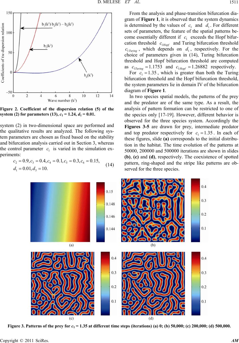

D. MELESE ET AL. 1511
From the analysis and phase-transition bifurcation dia-
gram of Figure 1, it is observed tha t the syste m dy na mic s
is determined by the valu es of 1 and 1. For different
sets of parameters, the feature of the spatial patterns be-
come essentially different if 1 exceeds the Hopf bifur-
cation threshold 1
c d
c
H
opf and Turing bifu rcation threshold
1Turing , which depends on 1
d, respectively. For the
choice of parameters given in (14), Turing bifurcation
threshold and Hopf bifurcation threshold are computed
as
c
3
c
c 1.175

and respectively.
1Turing 1Hopf
For 1
1.268c82
1.35c

, which is greater than both the Turing
bifurcation threshold and the Hopf bifurcation threshold,
the system parameters lie in domain IV of the bifurcation
diagram of Figure 1.
In two species spatial models, the patterns of the prey
and the predator are of the same type. As a result, the
analysis of pattern formation can be restricted to one of
the species only [17-19]. However, different behavior is
observed for the three species system. Accordingly the
Figures 3-5 are drawn for prey, intermediate predator
and top predator respectively for 1. In each of
these figures, slide (a) corresponds to the initial distribu-
tion in the habitat. The time evolution of the patterns at
50000, 200000 and 500000 iteration s are shown in slides
(b), (c) and (d), respectively. The coexistence of spotted
pattern, ring-shaped and the stripe like patterns are ob-
served for the three species.
1.35c
Figure 2. Coefficient of the dispersion relation (5) of the
system (2) for parameters (13), c1 = 1.24, d1 = 0.01.
system (2) in two-dimensional space are performed and
the qualitative results are analyzed. The following sys
e control parameter is varied in the simulation ex-
-
tem parameters are chosen as fixed based on the stability
and bifurcation analysis carried out in Section 3, whereas
th 1
periments:
23456
13
0.9, 0.4,0.1,0.3, 0.15,
0.01, 10.
ccccc
dd

 (14)
c
(a) (b)
(c) (d)
Figure 3. Patterns of the prey for c1 = 1.35 at different time steps (iterations) (a) 0; (b) 50,000; (c) 200,000; (d) 500,000.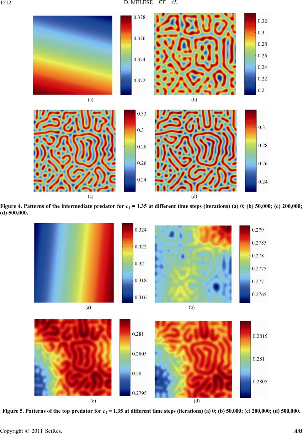

D. MELESE ET AL. 1512
(a) (b)
(c) (d)
Figure 4. Patterns of the intermediate preor for c1 = 1.35 at different time steps (iterations) (a) 0; (b) 50,000; (c) 200,000;
(d) 500,000.
dat
(a) (b)
(c) (d)
Figure 5. Patterns of the top predator for c 1.35 at different time steps (iterations) (a) 0; (b) 50,000; (c) 200,000; (d) 500,000.
1 =

D. MELESE ET AL. 1513
In Figure 3, one can see that the small spatial perturb-
bations to the homogeneous steady state of the spatio-
temporal system (2) leads to the formation of spots and
stripes of high prey density on a blue background of low
prey density (c.f. Figure 3(b)). However, at later time
some of the spots merge together to form stripes. This
results in an increase in the number of stripes and a de-
crease in the number of spots. Ring-shaped pattern is
also formed (c.f. Figures 3(c) and (d)).
The patterns of the intermediate predator shown in
Figure 4 is structurally similar wi
o
ic
ontrol parameter
th that of the patterns
f the prey shown in Figure 3. But, the background colo r
s not spatially uniform and varying temporally. In par- i
tular, the background density is decreasing with time.
The basic skeleton of the pattern of the top predator
(c.f. Figure 5) is similar with that of the patterns of the
prey and intermediate predator. However the background
density and the density in the patterns keep changing
spatially as well as temporally. Patches of different den-
sities are also visible.
Figure 6 shows the steady state patterns of the three
species for 11.24c. In this case, the c
1
c is greater than the Turing bifurcation threshold
1Turing
c but less than the Hopf bifurcation threshold
1
H
opf
c. That is, the parametric space is domain III of the
bifurcation diagram of Figure 1. This means that the
system has pure Turing instability and Turing patterns
ar
results show that the small spatial perturbations given to
the homogeneous steady state lead to the formation of
the stationary labyrinth like patterns. The density gradi-
ent of the prey is greater than that of the intermediate
predator and of the top predator. There is a sharp contrast
between two consecutive ribbons in the case of prey. The
contrast becomes progressively lower for intermediate
predator to top predator.
5. Conclusions
in region IV, both Turing and
opf instability occur and ring, stripe-like and spotted
In this study, the results show that the ratio-dependent
In this paper, we have presented a theoretical analysis of
evolutionary processes that involves organisms’ distribu-
tion and trophic interaction in spatially extended envi-
ronment with self diffusion. The numerical simulations
were consistent with the theoretical findings that there
are a range of parameters in 11
cd plane where the
different spatial patterns emerge. When the parameters
are located in region III of Figure 1, pure Turing insta-
bility occurs and labyrinth like patterns emerge. Whereas
when the parameters are
H
patterns coexist.
tri-trophic model with Michaelis–Menten type functional
response and diffusion represents rich spatial dynamics,
such as labyrinth pattern, coexistence of ring-shaped
pattern, spotted pattern and stripe-like pattern, which will
e expected for this choice. The numerical simulation
(b) (a)
(c)
Figure 6. Steady state patternop predator (c) for c1 = 1.24. s of the prey (a), intermediate predator (b) and t

D. MELESE ET AL. 1514
be useful for studying the dynamic complexity of eco-
systems or physical systems.
6. References
[1] A. Al-Khedhairi, “The Chaos and Control of Food Chain
Model Using Nonlinear Feedback,” Applied Mathemati-
cal Sciences, Vol. 3, No. 12, 2009, pp. 591-604.
[2] N. J. Gotelli and A. M. Ellison, “Food-Web Models Pre-
dict Species Abundances in Response to Habitat Change,”
PLoS Biology, Vol. 4, No. 10, 2006, pp. 1869-1873.
doi:10.1371/journal.pbio.0040324
[3] S. Gakkhar and R. K. Naji, “Chaos in Three Species Ra-
tio Dependent Food Chain,” Chaos, Solitons and Fractals,
Vol. 14, No. 5, 2002, pp. 771-778.
doi:10.1016/S0960-0779(02)00038-3
4] S. B. Hsu, T. W. Hwang[ and Y. Kuang, “A R
od Chain Model and Its Applications to
trol,” Mathematical Biosciences, Vol. 181,
No. 1, 2003, pp. 55-83.
atio-
Dependent Fo
Biological Con
doi:10.1016/S0025-5564(02)00127-X
[5] K. A. J. White and C. A. Gilligan, “Spatial Heterogeneity
in Three-Species, Plant-Parasite-Hyperparasite, Systems,”
Philosophical Transactions of Royal Society B, Vol. 353,
No. 1368, 1998, pp. 543-557.
doi:10.1098/rstb.1998.0226
[6] C. Neuhauser and S. W. Pacala, “An Explicitly Spatial
Version of Lotka-Voltera Model with Inter-Specific
Competition,” The Annals of Applied Probability, Vol. 9,
No. 4, 1999, pp. 1226-1259.
doi:10.1214/aoap/1029962871
[7] K. S. McCann, J. B. Rasmussen and J. Umbanhowar,
“The Dynamics of Spatially Coupled Food Webs,” Ecol-
ogy Letters, Vol. 8, No. 5, 2005, pp. 513-523.
doi:10.1111/j.1461-0248.2005.00742.x
Chon and T. Ma-[8] S. H. Lee, H. K. Pak, H. S. Wi, T. S.
tsumoto, “Growth Dynamics of Domain Pattern in a
Three-Trophic Population Model,” Physica A, Vol. 334,
No. 1-2, 2004, pp. 233-242.
doi:10.1016/j.physa.2003.11.017
eis and M. A. M. de Aguiar, [9] D. O. Maionchi, S. F. dos R
“Chaos and Pattern Formation in a Spatial Tritrophic
Food Chain,” Ecological Modelling, Vol. 191, No. 2,
2006, pp. 291-303. doi:10.1016/j.ecolmodel.2005.04.028
[10] M. Wang, “Stationary Patterns f
with Prey-Dependent and Rator a Prey-Predator Model io-Dependent Functional
Responses and Diffusion,” Physica D, Vol. 196, No. 1-2,
2004, pp. 172-192. doi:10.1016/j.physd.2004.05.007
[11] M. R. Garvie, “Finite-Difference Schemes for
Diffusion Equations Modeling Predator- Reac Prey Interactions
tion-
in MATLAB,” Bulletin of Mathematical Biology, Vol. 69,
No. 3, 2007, pp. 931-956.
doi:10.1007/s11538-006-9062-3
[12] A. B. Medvinsky, S. V. Petrovskii, I. A.
Malchow and B. L. Li, “Spatiote Tikhonov, H. mporal Complexity of
Plankton and Fish Dynamics,” SIAM Review, Vol. 44, No.
3, 2002, pp. 311-370.
doi:10.1137/S0036144502404442
[13] S. V. Petrovskii, B. L. Li and H. Malchow, “Transition to
Spatiotemporal Chaos Can Resolve the Paradox of En-
richment,” Ecological Complexity, Vol. 1, No. 1, 2004,
pp. 37-47. doi:10.1016/j.ecocom.2003.10.001
[14] H. Shen and Z. Jin, “Two Dimensional Pattern Formation
of Prey-Predator System,” Eighth ACIS International
Conference on Software Engineering, Artificial Intelli-
gence, Networking, and Parallel/Distributed Computing,
Qingdao, 30 July - 1 August 2007, pp. 343-346.
doi:10.1109/SNPD.2007.215
genesis,”
ol. 237,
[15] A. M. Turing, “The Chemical Basis of Morpho
Philosophical Transactions of Royal Society B, V
No. 641, 1952, pp. 37-72. doi:10.1098/rstb.1952.0012
[16] M. Banerjee and S.V. Petrovskii, “Self-Organized Spatial
Patterns and Chaos in a Ratio-Dependent Predator Prey
System,” Theoretical Ecology, Vol. 4, No. 1, 2011, pp.
37-53. doi:10.1007/s12080-010-0073-1
[17] W. Wang, L. Zhang, Y. Xue and Z. Jin, “Spatiotemporal
oral Com-
with Constant Harvest
Pattern Formation of Beddington-DeAngelis-Type Preda-
tor-Prey Model,” arXiv: 0801.0797v1 [q-bio.PE], January
2008.
[18] L. Zhang, W. Wang and Y. Xue, “Spatiotemp
plexity of a Predator-Prey System
Rate,” Chaos Solitons Fractals, Vol. 41, No. 1, 2009, pp.
38-46. doi:10.1016/j.chaos.2007.11.009
[19] W. Wang, Q. X. Liu and Z. Jin, “Spatiotemporal Com-
plexity of a Ratio-Dependent P
Physical Review E, Vol. 75, No.
redator-Prey System,”
5, 2007, Article ID
051913. doi:10.1103/PhysRevE.75.051913
[20] J. D. Murray, “Mathematical Biology II: Spatial Models
and Biomedical Applications,” Springer, Berlin, 2003.
G. Sun, Z. Jin, Q. X. Liu and L. Li, “Pattern Fo[21] rmation in
a Spatial S-I model with Nonlinear Incidence Rates,”
Journal of Statistical Mechanics: Theory and Experiment,
Vol. 2007, 2007, P11011.
doi:10.1088/1742-5468/2007/11/P11011
[22] H. Malchow, “Spatio-Temporal Pattern Formation in
Coupled Models of Plankton Dynamics and Fish School
Motion,” Nonlinear Analysis: Real World Applications,
Vol. 1, No. 1, 2000, pp. 53-67.
doi:10.1016/S0362-546X(99)00393-4
[23] S. B. L. Araújo and M. A. M. de Aguiar, “Pattern For-
mation, Outbreaks, and Synchronization in Food Chains
with Two and Three Species,” Physical Review E, Vol.
75, No. 6, 2007, Article ID 061908.
doi:10.1103/PhysRevE.75.061908
[24] W. Ko and I. Ahn, “Analysis of Ratio-Dependent Food
Chain Model,” Journal of Mathematical Analysis Appli-
cations, Vol. 335, No. 1, 2007, pp. 498-523.
doi:10.1016/j.jmaa.2007.01.089
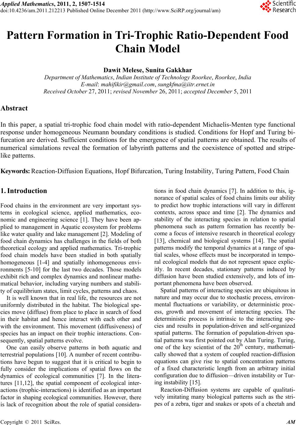