Psychology, 2010, 1: 22-26
doi:10.4236/psych.2010.11004 Published Online April 2010 (http://www.SciRP.org/journal/psych)
Analysis of Psychological Health and Life Qualities
of Internet Addicts Using Structural Equation
Model*
Qiaoling Tong1, Xuecheng Zou1, Yan Gong2, Hengqing Tong2
1Department of Electronic Science and Technology, Huazhong University of Science and T ech no lo gy, Wuhan, China; 2Department
of Mathematics, Wuhan University of Technology, Wuhan, China.
Received January 6th, 2010; revised January 28th, 2010; accepted January 29th, 2010.
ABSTRACT
Internet addiction disorder has become a serious social problem, and aroused great concern from the public and spe-
cialists. In this paper, the psychological states of internet addicts are measured by some famous mental scales, and their
life qualities are investigated by some questionnaires. Structural Equations Model (SEM) is used to analyze the rela-
tionship between the psychological health and life qualities of internet addicts. Meanwhile, a definite linear algorithm
of SEM is proposed which is useful for psychological analysis.
Keywords: Psychological Health, Life Quality, Internet Addict, SEM Algorithm
1. Introduction
Internet addiction disorder (IAD), or, more broadly,
Internet overuse, problematic computer use or patho-
logical computer use, is excessive computer use that
interferes with daily life. IAD was originally proposed
as a disorder in a satirical hoax by Ivan Goldberg in
1995 [1]. He took pathological gambling as diagnosed
by the Diagnostic and Statistical Manual of Mental
Disorders (DSM-IV) as his model for the description of
IAD [2]. It is not however included in the current DSM
as of 2009. IAD receives coverage in the press, and
possible future classification as a psychological disor-
der continues to be debated and researched.
Goldberg converted Internet Addiction Disorder (IAD)
into Pathological Computer Use (PCU). However, the
basic contents of these two are the same. This paper used
the concept of Internet Ad di ction.
Following Goldberg, people find their work could be
in trouble because of Intern et addiction, as well as social
relationship, family relationship, finance, psychology and
so on. Young (1996) discovered the emergence of a new
clinical disorder by Internet addiction [3]. Kraut (1998)
analyzed the Internet paradox: a social technology that
reduces social involvement and psychological well-being
[4]. Shaw (2002) analyzes the relationship between
Internet communication and depression, loneliness,
self-esteem, and perceived social support [5].
As the research go deep, mathematical models are
used to describe Internet addiction. Weiser (2001) builds
a cognitive-behavior model of pathological Internet ad-
diction (PIU). Zhang (2006) use Structural Equation
Model (SEM) to analyze the relationship of motives,
behaviors of Internet addiction and related social-
psychological health. Wen (2008) builds appropriate
standardized estimates for moderating effects in Struc-
tural Equation Models.
Indeed, SEM is very useful to investigate the personality
characteristic and life satisfaction of adults who have Inter-
net addiction, and reveal the relationships between them,
and the potential factor of Internet addiction. It will provide
basis to intervene the people with Internet addiction.
But there are some problems in calculation of SEM
because SEM is a indefinite equation. In this paper we
build a SEM for Internet addictio n, meanwhile we offer a
definite linear algorithm for SEM which is useful for any
SEM.
2. The Index System of Psychological Health
in Internet Addiction
The researches of Internet addiction vary from person to
person. Different people choose different scales. This
*The research was supported by the National Natural Science Founda-
tion of China
(
30570611, 60773210
)
.

Analysis of Psychological Health and Life Qualities of Internet Addicts Using Structural Equation Model 23
paper takes Young [3] ten questionnaires to inquiry In-
ternet addiction. There are many personality scales. Chi-
nese Minnesota Multiphasic Personality Inventory
(MMPI) which consists of ten indexes, including hypo-
chondriasis, depression, hysteria, psychopathic deviate,
masculinity feminity, paranoia, psychasthenia, schizo-
phrenia, hypomania and social introversion, is took to
test personality characteristic in this paper. Edward Di-
enner’s Life Satisfaction Scale is also adopted to test life
satisfaction, it comprises five questions.
The correlation between the above factors has been
given a clear description in some articles. These three
factors interact, and can be all affected by people’s basic
circs. We make an index system. People’s basic circs,
including sex, age, profession, education level, can be as
independent variables; meanwhile, we choose three de-
pendent variables which are Internet addiction, personal-
ity characteristic and life satisfaction. Independent vari-
able and three dependent variables are latent variables.
Each latent variable has certain kinds of explicit vari-
ables which are called manifest variables. The related
dependent variables are showed in Figure 1.
3. Structural Equation Model
Structural Equation Model (SEM) is a fast-growing
branch in the filed of applied statistics, widely used in
psychology, sociology and other fields. This paper is the
application of SEM to analyze social-psychological of
Internet addiction.
There are two kinds of equations in SEM. One is the
equations of the measurement model (outer model)
between the latent variables and the manifest variables,
we call Measurement Equations. The other is the equa-
tion of the structural model (inner model) among the
latent variables, we call Structural Equations. In our
model, there are 5 latent variables (1

, 2

, 13 ~

 )
and 5 path relationships. The path coefficients from the
exogenous latent variables i

to the endogenous la-
tent variables
j

are
j
i

, and the path coefficients
among the endogenous latent variables ij

are ij

.
Figure 1. The basic index of dependent var iable s
Structural Equation Model can also be seen as the
summary of secondary indicators. The latent variables
1

, 2

, 13 ~

are the first-level index, they are vir-
tual without direct observation values. Manifest vari-
ables are the second-level index, with practical obser-
vation values. The model in this paper, manifest vari-
ables can be acquired directly by questionnaire.
The Structural Equations are relationships among the
latent variables. The Structural Equations can be ex-
pressed as follows
1111
21 2222
1
31 32 3333
42 43 4444
0000
000
00
00

 


 



 


 
  
  
 
 
  

 
 
  
  
 
 
(1)
Under normal circumstances, the form of Structural
Equation coefficients may be different from the Equa-
tion (1) except for the diagonal line with 0. We use
vector and matrix to describe the Structural Equations.
Let 1 (, , )
k
 



, 1 (, ,)
m
 



. The coefficient
matrix of

is denoted as a mm matrix B, and
the coefficient matrix of

is denoted as a mk

matr ix

. The residual vector is


1
(, ,)
m



. The
Structural Equation (1) can be expressed as:
B




  (2)
The Measurement Equations are relationships be-
tween the latent variables and the manifest variables.
Suppose there are k exogenous latent variables and
m endogenous latent variables. The manifest variables
corresponding to the exogenous latent variable t

are
denoted as tj
x
, 1, ,tk

; 1,,( )jKt, where
()
K
t is the number of manifest variables correspond-
ing to the exogenous latent variable t

. The manifest
variables corresponding to the endogenous variable i

are denoted as ij y, 1, ,im

, 1,,( )jLi, where
()Li is the number of manifest variables correspond-
ing to the exogenous latent variable i

.
The Measurement Equations can be expressed as the
relationship from the manifest variables to the latent
variables:
()
1
Kt
ttjtjxt
j
x




, 1, ,tk (3)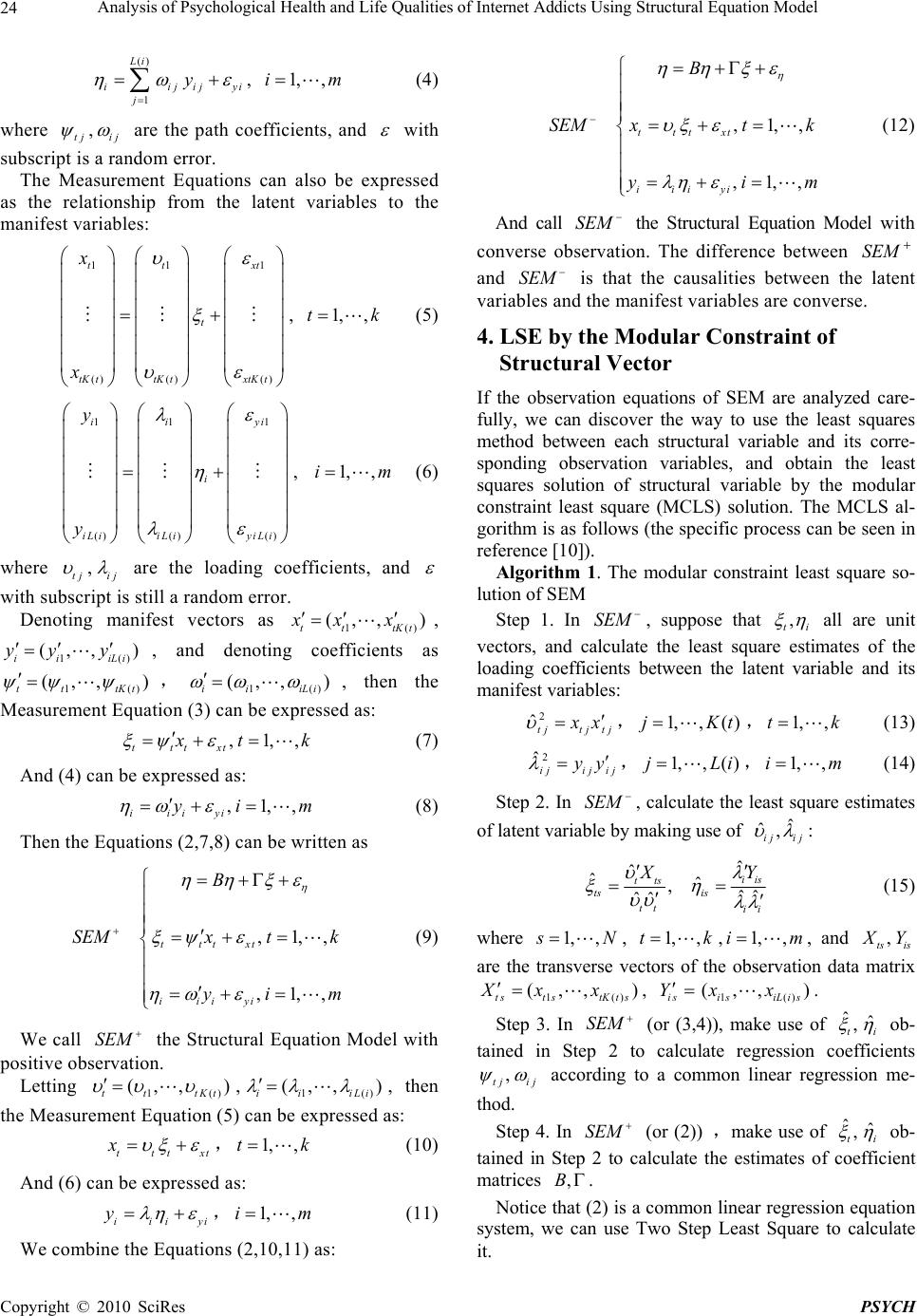

Analysis of Psychological Health and Life Qualities of Internet Addicts Using Structural Equation Model 24
()
1
Li
iijijyi
j
y




, 1,,im (4)
where tj

,ij

are the path coefficients, and

with
subscript is a random error.
The Measurement Equations can also be expressed
as the relationship from the latent variables to the
manifest variables:
11 1
() ()()
tt xt
t
tK ttKtxtKt
x
x



 
 
 
 

 
 
 
 
  , 1, ,tk (5)
11 1
() ()()
ii yi
i
iL iiL iyiL i
y
y



 
 
 
 

 
 
 
 
 
, 1, ,im (6)
where tj

,ij

are the loading coefficients, and

with subscript is still a random error.
Denoting manifest vectors as 1() (,, )
tt tKt
xx x
  ,
1()
(,, )
ii iLi
yy y
 
, and denoting coefficients as
1()
(,, )
tt tKt
 
，1()
(,, )
ii iLi


, then the
Measurement Equation (3) can be expressed as:
,1,,
tttxt
x
tk



   (7)
And (4) can be expressed as:
,1,,
iiiyi
yi m



  (8)
Then the Equations (2,7,8) can be written as
,1,,
,1,,
tttxt
iiiyi
B
SEMx tk
yi m


 
 





 








(9)
We call SEM  the Structural Equation Model with
positive observation.
Letting 1()
(,, )
tt tKt


,1()
(,, )
ii iLi


, then
the Measurement Equation (5) can be expressed as:
tttxt
x

 ，1, ,tk (10)
And (6) can be expressed as:
iiiyi
y

 ，1, ,im (11)
We combine the Equations (2,10,11) as:
,1,,
,1,,
tttxt
iiiyi
B
SEM xtk
yim


 
 




 


 




(12)
And call SEM

the Structural Equation Model with
converse observation. The difference between  SEM
and SEM

is that the causalities between the latent
variables and the manifest variables are converse.
4. LSE by the Modular Constraint of
Structural Vector
If the observation equations of SEM are analyzed care-
fully, we can discover the way to use the least squares
method between each structural variable and its corre-
sponding observation variables, and obtain the least
squares solution of structural variable by the modular
constraint least square (MCLS) solution. The MCLS al-
gorithm is as follows (the specific process can be seen in
reference [10]).
Algorithm 1. The modular constraint least square so-
lution of SEM
Step 1. In SEM

, suppose that ,
ti

 all are unit
vectors, and calculate the least square estimates of the
loading coefficients between the latent variable and its
manifest variables:
2
ˆtjtj tj
x
x 

，1,,()jKt

，1, ,tk (13)
2
ˆijij ij
yy 

，1,,( )jLi

，1, ,im (14)
Step 2. In SEM

, calculate the least square estimates
of latent variable by making use of ˆ
ˆ,
ij ij

 :
ˆ
ˆ,
ˆˆ
tts
ts
tt
X







ˆ
ˆˆˆ
iis
is
ii
Y





 (15)
where 1,,
s
N

, 1, ,tk

,1,,im, and ,
ts is
X
Y
are the transverse vectors of the observation data matrix
1()
(,,)
tst stK t s
Xx x


, is Y


1()
(,, )
is iLis
xx.
Step 3. In SEM

(or (3,4)), make use of ˆˆ ,
ti

 ob-
tained in Step 2 to calculate regression coefficients
,
tj ij

 according to a common linear regression me-
thod.
Step 4. In SEM

(or (2)) ，make use of ˆˆ
,
ti

 ob-
tained in Step 2 to calculate the estimates of coefficient
matrices ,B

.
Notice that (2) is a common linear regression equation
system, we can use Two Step Least Square to calculate
it.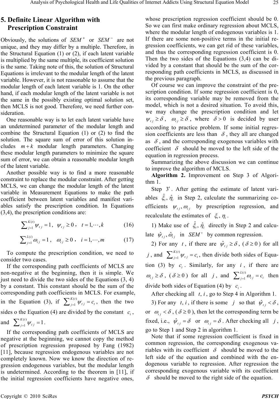

Analysis of Psychological Health and Life Qualities of Internet Addicts Using Structural Equation Model 25
5. Definite Linear Algor ithm with
Prescription Constraint
Obviously, the solutions of  SEM or  SEM are not
unique, and they may differ by a multiple. Therefore, in
the Structural Equation (1) or (2), if each latent variable
is multiplied by the same multiple, its coefficient solution
is the same. Taking note of this, the solution of Structural
Equations is irrelevant to the modular length of the latent
variable. However, it is not reasonable to assume that the
modular length of each latent variable is 1. On the other
hand, if each modular length of the latent variable is not
the same in the possibly existing optimal solution set,
then MCLS is not good. Therefore, we need further con-
sideration.
One reasonable way is to let each latent variable have
an undetermined parameter of the modular length and
combine the Structural Equation (1) or (2) to find the
solution. The square sum of error of this solution in-
cludes m
k
 modular length parameters. Changing
these modular length parameters to minimize the square
sum of error, we can obtain a reasonable modular length
of the latent variable.
Another possible way is to find a more reasonable
constraint to replace the modular constraint. After getting
MCLS, we can change the modular length of the latent
variable in Measurement Equations to make the path
coefficient between latent variables and manifest vari-
ables satisfy the prescription condition. In Equations
(3,4), the prescription conditions are:
()
11
Kt
tj
j


, 0
tj

，1, ,tk (16)
()
11
Li
ij
j


, 0 ij

，1, ,im (17)
To compute the prescription condition, we need to
consider two cases.
If the corresponding path coefficients of MCLS are
non-negative at the beginning, then it is simple. We
just need to divide the two sides of the Equations (3, 4)
by a constant. This constant should be the sum of the
corresponding path coefficients in MCLS. For example,
in the Equation (3), if ()
1
Kt
tj t
jc


, then the two
sides o the Equation (4) are divided by the constant t c,
and ()
11
Kt
tj
j


.
If the corresponding path coefficients of MCLS are
negative at the beginning, we cannot copy the method
of prescription regression proposed by Fang (1982)
[11], because regression endogenous variables are not
completely known. Now we know the direction of re-
gression endogenous variables, but the modular length
is undetermined. According to the theorem in [11], if
the initial regression coefficients have negative ones,
whose prescription regression coefficient should be 0.
So we can first make ordinary regression about MCLS,
where the modular length of endogenous variables is 1.
If there are some non-positive terms in the initial re-
gression coefficients, we can get rid of these variables,
and thus the corresponding regression coefficient is 0.
Then the two sides of the Equations (3,4) can be di-
vided by a constant that should be the sum of the cor-
responding path coefficients in MCLS, as discussed in
the previous paragraph.
Of course we can improve the constraint of the pre-
scription condition. If some regression coefficient is 0,
its corresponding variable may be removed from the
model, which is not a desired situation. To avoid this,
we may change the prescription condition and let
tj

 , ij

 , where 0

 is decided by user
according to practice problem. If some initial regres-
sion coefficients are less than

, they all are changed
as

, and the corresponding exogenous variables with
coefficien t

should be moved to the left side of the
equation in regression process.
Summarizing the above discussion we can continue
to improve the algorithm of MCLS.
Algorithm 2. Improvement on Step 3 of Algori-
thm 1.
Step 3

. After getting the estimate of latent vari-
ables ˆˆ ,
ti

 in Step 2, calculate the summarizing co-
efficien ts ,
tj ij

 by prescription regression, and
recalculate the estimates of ,
ti

 .
1) Make use of ˆˆ
,
ti

 directly in Step 2 and calcu-
late ˆˆ ,
tj ij

 in SEM

b y common regression.
2) For any t, if there are ˆtj

 , (0

) for all
j, and ()
1
Kt
tj t
jc



, then divide both sides of Equa-
tion (3) by t c. Similarly, for any i, if there are
ij

 , (0

) for all j, and ()
1
Li
ij i
jc



 then
divide both sides of Equation (4) by i c.
After checking all ,ti, go to Step 4 in Algorithm 1.
3) For any ,ti, if there is some j so that ˆtj



,
or ij



, (0

), then let the corresponding term be
fixed, i.e., ˆtj



or ij

 . After checking all j,
go to Step 1 and Step 2 in algorithm 1.
Note that if some regression coefficient is fixed in
common regression, the corresponding exogenous va-
riables with its coefficient

should be moved to the
left side of the equation and combined with the en-
dogenous variable to regression. After regression the
corresponding exogenous variable with its coefficient

should be moved to the right side of the equation.

Analysis of Psychological Health and Life Qualities of Internet Addicts Using Structural Equation Model 26
This model and definite algorithm is helpful to re-
searchers who study Internet addiction. More detailed
proof of algorithm and data examples can be found in
website http://public.whut.edu.cn/slx/English/.
6. Acknowledgment
The authors would like to express sincerely thanks to the
referees and editors for their valuable comments.
REFERENCES
[1] I. Goldberg, “Internet Addiction Disorder,” 1995. http://
www.cog.brown.edu/brochure/people/duchon/humor/inte
rnet.addiction.html
[2] J. J. Block, “Issues for DSM-V: Internet Addiction,”
American Journal of Psychiatry, Vol. 165, No. 3, 2008,
pp. 306-307.
[3] K. S. Young, “Internet Addiction: The Emergence of a
New Clinical Disorder,” Cyber Psychology and Behavior,
Vol. 3, 1996, pp. 237-244.
[4] R. Kraut, M. Patterson, V. Lundmark, S. Kiesler, T. Mu-
kophadhyay and W. Scherlis, “Internet Paradox: A Social
Technology that Reduces Social Involvement and Psy-
chological Well-Being,” American Psychologist, Vol. 53,
No. 9, 1998, pp. 1017-1031.
[5] L. H. Shaw and L. M. Gant, “In Defense of the Internet:
The Relationship between Internet Communication and
Depression, Loneliness, Self-Esteem and Perceived So-
cial Support,” Cyber Psychology and Behavior, Vol. 5,
No. 2, 2002, pp. 157-171.
[6] E. B. Weiser, “The Function of Internet Addiction and
Their Social and Psychological Consequences,” Cyber
Psychology and Behavior, Vol. 4, No. 6, 2001, pp. 723-
743.
[7] R. A. Davis, “A Cognitive-Behavioal Model of Patho-
logical Internet Addiction (PIU),” Computers in Human
Behavior, Vol. 17, 2001, pp. 87-195.
[8] F. Zhang, M. Shen, M. Xu, H. Zhu and N. Zhou, “A
Structural Equation Modeling of Motives, Behaviors of
Internet Addiction and Related Social-Psychological
Health,” Acta Psychological Sinica, Vol. 38, No. 3, 2006,
pp. 407-413.
[9] Z. Wen, J. Hou and W. M. Herbert, “Appropriate Stan-
dardized Estimates for Moderating Effects in Structural
Equation Models,” Acta Psychological Sinica, Vol. 40,
No. 6, 2008, pp. 729-736.
[10] C. Wang and H. Tong, “Best Iterative Initial Values for
PLS in a CSI Model,” Mathematical and Computer Mod-
elling, Vol. 46, No. 3-4, 2007, pp. 439-444.
[11] K. T. Fang, D. Q. Wang and G. F. Wu, “A Class of Con-
straint Regression-Fill a Prescription Regression,” Mathe-
matica Numerica Sinica, Vol. 4, 1982, pp. 57-69.